DB 내부 ⑪: SQL 실행기, 텍스트에서 행까지, 조인 3형제와 3값 논리
목차
0. 들어가며: 선언형 언어가 행이 되기까지
이 시리즈의 1~10편은 저장·복구·격리·최적화·분산을 다뤘는데, 정작 한 축이 비어 있었습니다. SQL 텍스트가 실제 행이 되기까지의 실행기 파이프라인 그 자체입니다. 이 편이 그 축을 완결합니다.
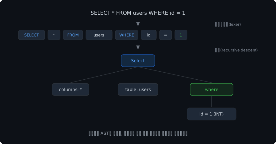
SQL은 선언형 언어입니다. “무엇을”만 말하고 “어떻게”는 안 말합니다. SELECT * FROM users WHERE id = 1이라는 문자열이 힙의 실제 행이 되려면 세 단계가 필요합니다.
SQL 텍스트 → [렉서] → 토큰 → [파서] → AST → [실행기] → 행컴파일러의 앞단을 그대로 빌려온 구조입니다. 모든 DB의 프런트엔드가 이렇게 생겼습니다. 실제 DB는 AST와 실행기 사이에 분석(analyze)·재작성(rewrite)·계획(plan) 단계가 더 있습니다(6편이 그 계획 단계). 이 편이 다루는 건 그 앞뒤의 양 끝단입니다.
1. 렉서: 글자를 토큰으로
1단계는 토크나이저(렉서). SELECT * FROM users WHERE id = 1 → [SELECT] [*] [FROM] [IDENT:users] [WHERE] [IDENT:id] [=] [INT:1]. 하는 일은 공백 건너뛰기, 글자 덩어리 묶기, '...' 문자열 떼기, 그리고 미묘한 규칙 하나입니다:
/* 비교 연산자: 두 글자를 먼저 본다 */if (c == '<' && nx == '=') { ...; t.type = TOK_LE; } /* <= */if (c == '<' && nx == '>') { ...; t.type = TOK_NE; } /* SQL의 <> */if (c == '<') { ...; t.type = TOK_LT; } /* 그냥 < */maximal munch:
<=를 만났을 때<하나만 떼면 뒤의=가 엉뚱하게 따로 떨어진다. 렉서는 “가능한 한 긴 토큰을 먼저 집는다”(longest match). 거의 모든 렉서의 원칙이다.
키워드와 식별자의 구분도 여기서 정해집니다. 덩어리를 다 읽은 뒤 예약어 표를 조회해서(strcasecmp로 대소문자 무시) users는 IDENT, FROM은 키워드 토큰이 됩니다.
실무/면접 포인트, 예약어는 왜 생기나:
SELECT가 키워드 토큰이 되므로 컬럼 이름으로 그냥select를 쓰면 파서가 헷갈린다. 그래서 예약어(reserved word)가 존재하고, 따옴표로 escape하면 쓸 수 있다. PostgreSQL은"select", MySQL은 백틱, SQL Server는[select]. 진짜 DB는 비예약(non-reserved) 키워드도 둬서 일부는 그냥도 허용한다.
2. 재귀 하강 파서: 문법 규칙 하나 = 함수 하나
2단계는 파서. 토큰을 트리(AST)로 조립합니다. 재귀 하강(recursive descent)의 묘미는 문법 규칙 하나하나가 함수 하나가 된다는 것입니다. 파서 코드가 거의 영어로 읽힙니다.
static void parse_select_stmt(Parser *p, SelectStmt *s) { parse_select_list(p, s); /* * 또는 컬럼/집계 목록 */ p_expect(p, TOK_FROM, "FROM이 필요합니다"); parse_name(p, s->table); if (p_accept(p, TOK_WHERE)) parse_where(p, &s->where); if (p_accept(p, TOK_GROUP)) { /* GROUP BY ... */ } if (p_accept(p, TOK_ORDER)) { /* ORDER BY ... */ }}파서를 떠받치는 도구는 셋뿐입니다. p_accept(있으면 소비, 선택 문법), p_expect(없으면 에러, 필수 문법), p_advance(다음 토큰)입니다. 이 셋이 재귀 하강의 전부라 해도 됩니다.
두 가지가 특히 배울 지점입니다.
- 우선순위 = 함수 호출 순서. WHERE는
term (OR term)*, term은cond (AND cond)*로 파싱됩니다. AND가 OR보다 안쪽 함수라a AND b OR c는 자연히(a AND b) OR c가 됩니다. 연산자 우선순위를 표가 아니라 호출 구조로 표현하는 것입니다. - 서브쿼리에서 파서가 자기 자신을 부른다.
WHERE id IN (SELECT ...)를 만나면 조건 파싱 함수 안에서parse_select_stmt를 다시 부릅니다. 문법이 재귀적이니 파서도 재귀적입니다. “재귀 하강”이라는 이름의 정체입니다(AST의Condition이SelectStmt*를 품는 자기참조 구조가 됩니다).
손으로 쓴 파서 vs 파서 생성기
| 손으로 쓴 재귀 하강 | 파서 생성기 (yacc/bison) | |
|---|---|---|
| 문법 정의 | 함수로 직접 (코드 = 문법) | 별도 .y 문법 파일 |
| 에러 메시지 | 마음대로 (위치·맥락 자유) | 기본값에 갇히기 쉬움 |
| 디버깅 | 함수 따라가기 | 생성된 상태 머신을 봐야 |
| 큰 문법·복잡한 우선순위 | 함수가 늘어남 | 빛난다 (자동 처리) |
| 채택 | GCC/Clang, MSVC | MySQL(bison), PostgreSQL(bison), SQLite(자체 LALR(1) 생성기 Lemon) |
PostgreSQL과 MySQL은 bison(LALR 생성기)을 쓰고, SQLite도 자체 LALR(1) 생성기 Lemon으로 파서를 생성합니다. 주요 DB의 파서는 생성기 쪽이 대세입니다. 손 파서는 에러 메시지와 디버깅 통제가 쉬워 컴파일러 세계(GCC/Clang/MSVC)에선 오히려 주류입니다. 학습용으로도 “코드가 곧 문법”이라 압도적으로 유리합니다.
3. 실행기: 스트리밍과 materialize가 갈리는 곳
3단계, AST를 힙 연산으로. 실행기의 큰 그림은 연산자 트리를 행이 흐르는 파이프라인으로 보는 Volcano/iterator 모델입니다. 연산자마다 open·next·close를 두는 tuple-at-a-time 반복자 방식의 정식화가 Graefe(1994)입니다. (발명이 아니라 정식화입니다. open-next-close 인터페이스 자체는 System R 계열부터 쓰였고, PostgreSQL 실행기도 Berkeley POSTGRES(1986~) 시절부터 이 반복자 모델을 따릅니다.) 미니 DB는 이를 콜백(visit) 스타일로 단순화했지만, 본질적 구분 하나는 그대로 드러납니다:
행이 흐르는 방식은 셋으로 갈린다. ① 스트리밍:
WHERE는 행 하나로 통과/탈락이 정해지니 한 행씩 흘려보내면 된다. ② blocking이지만 상태는 작음:COUNT(*)같은 집계는 마지막 행까지 소비해야 결과를 낼 수 있지만(blocking), 행을 쌓아 둘 필요는 없다. 누산기만 갱신하면 되고 메모리는 O(그룹 수)다. ③ 진짜 materialize:ORDER BY는 정렬할 행 전체를 적재해야 한다. 이 구분이 메모리 사용량과 첫 행 응답 시간을 가른다.
이 구분은 이미 시리즈 곳곳에서 일했습니다. 8편의 병렬화가 스트리밍 SELECT와 집계를 다른 전략으로 다룬 이유가 이것입니다. 그리고 고백 하나. 미니 DB의 집계는 ②를 ③처럼 구현했었습니다. 누산기 대신 행을 4,096행 버퍼에 모은 뒤 계산하는 방식이었고, 그 버퍼 상한이 바로 8편의 silent 버그(6,000행 테이블에 COUNT가 에러 없이 4096)를 낳았습니다. 실제 DB의 집계 노드는 행을 버퍼링하지 않고 누산기만 흘립니다. ②와 ③을 섞으면 안 되는 이유를 버그로 배운 셈입니다.
Volcano 이후의 이야기도 한 단락만 덧붙입니다. tuple-at-a-time은 행마다 함수 호출·분기 비용이 붙어 분석(OLAP) 워크로드에선 비쌉니다. 그래서 DuckDB·ClickHouse는 수천 행 단위 벡터(배치) 로 흘리는 벡터화 실행을 택했고, PostgreSQL은 11부터 표현식 평가를 JIT 컴파일하는 길을 더했습니다. 모델의 뼈대(연산자 트리를 흐르는 데이터)는 그대로고, “한 번에 몇 행씩”이 바뀐 겁니다.
4. 조인 3형제: 모든 조인은 이중 루프에서 시작한다
여러 테이블을 잇는 조인의 출발점은 중첩 루프 조인(NLJ) 입니다. 바깥 테이블을 한 행씩 훑으며, 행마다 안쪽 테이블을 전부 스캔해 ON이 맞는 짝을 붙이는 이중 루프입니다.
핵심 사실: 모든 조인 알고리즘의 출발점은 중첩 루프다. “맞는 짝을 찾는다”의 가장 솔직한 표현이고, 인덱스·해시·정렬병합은 전부 이 안쪽 루프를 빠르게 만드는 변형일 뿐이다.
- 인덱스 NLJ: 안쪽 테이블의 조인 키에 인덱스가 있으면, 안쪽 전체 스캔 대신 바깥 행의 키로 점 조회. O(N×M) → O(N×log M).
- 해시 조인: 안쪽을 한 번 훑어
조인 키 → 행 목록해시를 만들고(build), 바깥을 한 번 훑으며 조회(probe). O(N×M) → O(N+M), 인덱스가 없어도. 단 등식 조인만 됩니다(해시는 순서가 없으니까). - 정렬 병합 조인: 양쪽을 조인 키로 정렬해 지퍼 잠그듯 나란히 훑기. 미니 DB는 안 만들었습니다. 정렬 인프라가 더 필요하고 우리 규모에선 보여줄 게 적어서(정직한 생략).
| NLJ | 인덱스 NLJ | 해시 조인 | 정렬 병합 | |
|---|---|---|---|---|
| 복잡도 | O(N×M) | O(N×log M) | O(N+M) | O(정렬+N+M) |
| 조인 조건 | 아무거나 | 인덱스가 지원하는 비교(등식·범위) | 등식만 | 등식(이론상 범위 band join도 가능하나 PG의 Merge Join은 사실상 등식) |
| 사전 준비 | 없음 | 인덱스 | 해시 빌드(메모리) | 양쪽 정렬 |
| 빛나는 곳 | 한쪽이 아주 작을 때 | OLTP(안쪽에 인덱스) | 양쪽 크고 정렬 안 됨(OLAP) | 이미 정렬됐거나 해시가 메모리 초과 |
미니 DB는 조인 레벨마다 “안쪽 PK가 조인 키면 인덱스 NLJ, 그 밖의 등식이면 해시, 아니면 스캔”으로 고릅니다. 6편의 비용 모델이 이 선택을 정교화한 것입니다. PostgreSQL은 여기에 정렬 병합까지 셋을 비용(work_mem에 해시가 들어가나, 어느 쪽이 이미 정렬돼 있나)으로 저울질합니다.
실무/면접 포인트: “해시 조인은 왜 등식만 되나”의 본질입니다. 해시는 순서를 버리는 대가로 O(1) 조회를 얻는 구조입니다. 범위 비교에는 순서가 필요하니 양립 자체가 불가능하고, 해시 인덱스가 범위 스캔을 못 하는 것과 같은 뿌리입니다. “자료구조가 무엇을 버렸는지”가 곧 “어떤 연산을 못 하는지”입니다.
LEFT JOIN과 NULL의 등장. INNER는 맞는 쌍만 내보내지만, LEFT는 왼쪽 행을 매칭이 없어도 살리고 오른쪽을 NULL로 채웁니다. 구현은 “이번 바깥 행이 매칭됐나” 플래그 하나입니다. 그리고 이 NULL 채움이 인덱스/해시/스캔 어느 방법과도 직교한다는 게 설계의 미덕입니다(방법 선택과 NULL 로직이 서로 안 얽힘).
5. 집계: GROUP BY는 왜 정렬(또는 해시)인가
WHERE가 행을 거르고 조인이 행을 잇는다면, GROUP BY+집계는 여러 행을 하나로 접습니다. 처음으로 “행 하나 → 행 하나”가 아닌 연산입니다. 한 그룹의 COUNT는 그 그룹 전체를 봐야 나오니, 같은 그룹의 행들이 인접해야 구간 단위로 누산기를 돌릴 수 있습니다. 그래서 길이 둘입니다:
- 정렬 기반(GroupAggregate): 그룹 키로 정렬하면 같은 키가 연속 구간이 된다. 미니 DB와 PostgreSQL의 GroupAggregate 방식(PG는 입력이 이미 정렬돼 있으면 모으지 않고 스트리밍).
- 해시 기반(HashAggregate): 그룹 키 → 누산기 해시를 두고 한 번에 스캔. 정렬이 필요 없지만 그룹 수만큼 메모리를 쓴다. PostgreSQL에선 그 한도가
work_mem × hash_mem_multiplier이고, 13부터는 실행 중 한도를 넘어도 죽거나 계획을 못 바꾸는 대신 디스크로 spill해 계속 간다. PostgreSQL이 둘을 비용으로 고른다.
HAVING은 그룹의 WHERE입니다. WHERE가 그룹핑 전에 개별 행을 거르고, HAVING이 집계가 끝난 뒤에 그룹을 거릅니다(HAVING COUNT(*) > 2). 적용 시점이 다르다는 것이 둘의 전부입니다.
이 “적용 시점”을 문장 전체로 넓힌 것이 SQL의 논리적 평가 순서입니다. 적는 순서(SELECT가 맨 앞)와 달리, 의미는 FROM → WHERE → GROUP BY → HAVING → SELECT → ORDER BY 순으로 정의됩니다. WHERE에서 SELECT의 별칭을 못 쓰는 이유가 이것입니다. 별칭은 SELECT 단계에서야 생기기 때문입니다. 별칭을 볼 수 있는 절은 SELECT 뒤에 오는 ORDER BY뿐입니다. (어디까지나 의미의 순서입니다. 실제 실행 계획은 결과만 같으면 얼마든지 재배열합니다.)
흔한 오해 정정: “COUNT(1)이 COUNT()보다 빠르다?”* PostgreSQL과 MySQL(InnoDB)에서 둘은 사실상 동등합니다.
COUNT(*)는 “모든 컬럼을 읽어라”가 아니라 “행 수를 세라”는 전용 의미라 컬럼을 볼 필요조차 없고, PostgreSQL에선 오히려COUNT(*)가 더 잘 최적화된 경로를 탑니다.*를 컬럼 목록으로 읽은 직관이 이 미신의 뿌리인데, 여기서*는 문법 기호일 뿐입니다.
6. WHERE의 확장: 공짜인 것과 아닌 것
기능을 얹을 때마다 “새 코드가 필요한가”가 갈렸는데, 그 갈림 자체가 배울 거리입니다.
BETWEEN, 실행기 0줄 (문법 설탕). col BETWEEN a AND b는 파서가 그 자리에서 (col >= a) AND (col <= b)로 풀어버리면 끝입니다. 실행기는 자기가 BETWEEN을 처리하는 줄도 모릅니다. (PostgreSQL은 파스 트리에 BETWEEN 노드를 남겼다가 나중에 변환합니다. 어디서 푸느냐는 구현 선택입니다.) IN (v1, v2, ...)도 같은 결입니다. 값 집합 멤버십일 뿐입니다.
LIKE, 진짜 새 연산자. %(0글자 이상)·_(한 글자) 와일드카드는 어떤 기존 비교로도 안 풀립니다. 매칭 알고리즘의 갈림길이 셋인데:
| 방식 | 시간 | 공간 | 문제 |
|---|---|---|---|
| 재귀 | 최악 지수적 | 스택 | % 여러 개면 호출 폭발 |
| DP 테이블 | O(n·m) | O(n·m) | 길이 곱만큼 메모리 |
| 백트래킹 two-pointer | 평균 ~O(n) | O(1) | 인위적 최악 패턴에서 출렁임 |
static int like_match(const char *s, const char *pat) { const char *star = NULL, *ss = NULL; while (*s) { if (*pat == '%') { star = pat++; ss = s; } /* %: 위치 기억, 일단 0글자 */ else if (*pat == '_' || *pat == *s) { pat++; s++; } /* 한 글자 일치 */ else if (star) { pat = star + 1; s = ++ss; } /* 막힘 -> %가 한 글자 더 먹은 셈 */ else return 0; } while (*pat == '%') pat++; return *pat == '\0';}포인터 둘과 “마지막 % 위치”만 기억하는 O(1) 공간 매처입니다.
실무/면접 포인트, LIKE ‘%x%‘는 왜 느린가: 인덱스는 값을 정렬한 구조라,
'kim%'처럼 앞이 고정된 패턴만 “정렬된 구간의 시작점”으로 점프할 수 있다. 앞이%로 열리면 시작점을 특정할 수 없어 풀 스캔이다. 미니 DB만이 아니라 B-tree 인덱스의 본질적 한계다. 중간 일치가 필요하면 인덱스 자체를 바꾼다: PostgreSQL의 트라이그램(pg_trgm, 문자열을 3글자 조각으로 쪼개 색인), 또는 검색 엔진의 역색인(Lucene/Elasticsearch).
흔한 오해 정정: “접두 LIKE는 인덱스를 탄다?” PostgreSQL에선 조건이 하나 더 붙습니다. 기본(비-C) collation으로 만든 일반 btree 인덱스는
LIKE 'kim%'조차 못 탑니다. locale의 문자열 비교 규칙이 바이트 순서와 달라서, “kim으로 시작”을 “정렬된 한 구간”으로 변환할 수 없기 때문입니다.text_pattern_ops연산자 클래스로 인덱스를 만들거나 C collation을 써야 접두 LIKE가 인덱스를 탑니다(PostgreSQL 문서 Operator Classes). “앞이 고정이면 된다”는 원리 위에 collation이라는 현실이 한 겹 더 있는 겁니다.
타입 강제 변환: WHERE age = '30'은 무슨 일을 하나. 비교의 양변 타입이 다를 때 DB가 얼마나 관대하게 변환해 주느냐는 제품마다 완전히 다릅니다:
| PostgreSQL | MySQL | SQLite | |
|---|---|---|---|
| 철학 | 명시적: 정해진 캐스트 규칙만, 안 되면 에러 | 관대: 암묵 변환을 넓게 허용 | type affinity: 컬럼의 “선호 타입”으로 저장 시점에 변환 |
'1abc' + 1 | 에러 | 2 + warning (앞자리 숫자만 파싱) | 문맥에 따라 2 |
| 실패 방식 | 일찍, 시끄럽게 | 조용히 이상한 결과 | 스키마가 타입을 강제하지 않음 |
미니 DB는 타입이 INT/TEXT 둘뿐이라 이 문제를 비켜갔지만, 실무의 함정은 의미만이 아니라 성능 쪽에도 있습니다.
실무 안티패턴: 인덱스 컬럼을 다른 타입의 값과 비교하는 것. 변환이 컬럼 쪽에 걸리는 순간 인덱스가 무력화됩니다. 예컨대 MySQL에서 문자열 컬럼을 숫자와 비교하면 컬럼 값이 행마다 숫자로 변환되며 풀 스캔이 됩니다. 전형적인 발생 경로가 애플리케이션의 파라미터 바인딩 타입 불일치(문자열 컬럼에 숫자 파라미터를 바인딩)입니다. 코드도 SQL도 멀쩡해 보이고, EXPLAIN을 떠 봐야 드러납니다.
서브쿼리, uncorrelated는 한 번만 돈다. IN (SELECT uid FROM orders)의 안쪽은 바깥 행과 무관하니, 바깥 스캔 전에 한 번 돌려 값 집합을 캐시하고 바깥은 멤버십만 검사합니다. 행마다 재실행하면 O(행×서브쿼리), 캐시하면 O(행)입니다. 이 구분(uncorrelated vs correlated)이 진짜 옵티마이저의 서브쿼리 unnesting이 하는 고민의 출발점입니다. 그리고 8편에서 서브쿼리 WHERE가 병렬화 게이트에 걸렸던 이유도 이것입니다. 술어가 실행기를 재진입하기 때문입니다.
7. NULL의 의미론: 3값 논리
1편에서 NULL의 저장(비트맵)을 다뤘으니, 여기선 의미를 닫습니다. SQL의 비교는 참/거짓이 아니라 3값, 곧 TRUE / FALSE / UNKNOWN입니다.
핵심 규칙: NULL은 “값이 없음”이 아니라 “모름” 이다. 모르는 것과의 비교는 그 결과도 모른다.
NULL = NULL은 TRUE가 아니라 UNKNOWN이다(둘 다 모르는 값인데 같은지 어떻게 아나). 그리고 WHERE는 TRUE만 통과시킨다. UNKNOWN은 FALSE처럼 걸러진다.
이 두 줄에서 실무의 함정들이 전부 유도됩니다:
WHERE col = NULL은 아무 행도 안 나온다 (전부 UNKNOWN). NULL 검사는 전용 연산자IS NULL/IS NOT NULL로. PostgreSQL 문서가 명시적으로 경고하는 지점입니다. “Do not write expression = NULL because NULL is not ‘equal to’ NULL.”NOT IN+ NULL 함정:x NOT IN (1, NULL)은x != 1 AND x != NULL인데 뒤가 UNKNOWN이라 전체가 최고 UNKNOWN이다. 절대 TRUE가 될 수 없어 결과가 통째로 빈다. 서브쿼리 결과에 NULL이 하나만 섞여도NOT IN이 전멸하는 유명한 사고. 대칭 케이스도 미묘합니다.x IN (1, NULL)은 x=1이면 TRUE지만, x≠1이면 FALSE가 아니라 UNKNOWN입니다(x = NULL이 UNKNOWN이라 OR 전체가 UNKNOWN). WHERE에선 어차피 걸러져 티가 안 나다가, NOT으로 뒤집는 순간 위의 함정이 되는 구조입니다.- 집계는 NULL을 건너뛴다:
COUNT(*)는 행 수(NULL 포함),COUNT(col)/SUM/AVG는 비NULL만.AVG의 분모도 비NULL 개수다. 이 구분은 8편의 부분 집계에서 누산기를 둘로 나눈 이유였다. - 정렬에서 NULL의 자리: 비교가 안 되니 위치를 정해줘야 한다. PostgreSQL은 기본 NULLS LAST(ASC 기준)이고 지정도 가능하다. 미니 DB도 같은 기본값이다.
정렬 기본값은 DB마다 달라서, 이식할 때 물어봐야 하는 항목입니다:
| 기본 위치 (ASC) | NULLS FIRST/LAST 문법 | |
|---|---|---|
| PostgreSQL | NULLS LAST | 있음 |
| MySQL | NULL을 최솟값 취급 → 먼저 | 없음 (ORDER BY col IS NULL 트릭으로 우회) |
| SQLite | 최솟값 취급 → 먼저 | 3.30부터 있음 |
실무 안티패턴: nullable 컬럼을 서브쿼리로 걸러야 할 때
NOT IN (SELECT ...)을 쓰는 것. 서브쿼리 결과에 NULL이 하나라도 있으면 결과가 통째로 비고(의미), 옵티마이저도 anti-join으로 풀기 어려워집니다(성능). 이중으로 손해입니다.NOT EXISTS는 NULL에 이 함정이 없고 anti-join으로 잘 풀립니다. nullable이 끼면 기본값은NOT EXISTS입니다. 면접에서 “NOT IN vs NOT EXISTS”를 받으면, 성능 전에 NULL이 있으면 결과 자체가 다르다부터 답하는 게 정확한 순서입니다.
그런데 SQL이 NULL을 언제나 “모름”으로 일관되게 다루느냐 하면, 아닙니다. 구문마다 태도가 갈립니다:
- GROUP BY / DISTINCT는 NULL들을 한 그룹으로 묶습니다. 비교 기준이 equality가 아니라 “not distinct”이기 때문입니다(NULL은 NULL과 not distinct).
- UNIQUE 제약은 반대로 NULL들을 서로 다른 값처럼 취급해 여러 행을 허용합니다. PostgreSQL의 기본이고, 15부터는
NULLS NOT DISTINCT로 바꿀 수 있습니다. SQL Server는 기본이 반대(NULL 1개만 허용). - CHECK 제약은 UNKNOWN을 통과시킵니다. PostgreSQL 문서의 표현으로 “satisfied if the check expression evaluates to true or the null value.” WHERE(UNKNOWN 탈락)와 정반대 방향입니다.
흔한 오해 정정: “NULL은 그냥 특별한 값이다?” 값이라면 모든 구문에서 같은 규칙을 따라야 할 텐데, 비교에선 UNKNOWN을 낳고, GROUP BY에선 한 그룹이고, UNIQUE에선 서로 다르고, CHECK은 통과시킵니다. NULL은 하나의 값이 아니라 구문마다 다르게 답하는 “부재의 표시” 에 가깝습니다. 그래서 nullable 컬럼이 낀 로직은 구문별 규칙을 하나씩 확인해야 합니다.
8. 정리: 시리즈의 실행기 축, 완결
- 파이프라인: 렉서(maximal munch, 예약어) → 재귀 하강 파서(문법=함수, 우선순위=호출 구조, 서브쿼리=자기 재귀) → 실행기(스트리밍 / blocking / materialize).
- 조인 3형제: 전부 중첩 루프의 변형. 인덱스는 안쪽을 점 조회로, 해시는 O(N+M)으로(등식만), 정렬 병합은 정렬된 입력에서. LEFT JOIN의 NULL 채움은 방법 선택과 직교.
- 집계: 같은 그룹이 인접해야 접을 수 있다. 정렬 기반(GroupAggregate) vs 해시 기반(HashAggregate). HAVING = 그룹의 WHERE.
- 공짜 vs 진짜: BETWEEN/IN(목록)은 파서의 문법 설탕(실행기 0줄), LIKE는 진짜 새 연산자(O(1) 공간 백트래킹 매처).
'%x%'가 느린 건 B-tree의 본질이다. 탈출구는 트라이그램·역색인. - 3값 논리: NULL은 “모름”, WHERE는 TRUE만 통과.
NOT IN+NULL 전멸,COUNT(*) vs COUNT(col), NULLS LAST가 전부 여기서 유도된다. 단 GROUP BY(한 그룹)·UNIQUE(서로 다름)·CHECK(통과)은 각자 다른 규칙이다. NULL은 구문마다 태도가 갈린다.
이로써 시리즈가 진짜 완결입니다. 저장(①)부터 실행기(⑪)까지, 미니 DB가 가진 모든 축을 다뤘습니다.
참고 (1차 자료 우선)
- Goetz Graefe, Volcano — An Extensible and Parallel Query Evaluation System (IEEE TKDE, 1994)
- PostgreSQL Documentation: The Parser Stage
- PostgreSQL Documentation: Pattern Matching (LIKE, pg_trgm)
- SQLite: The Lemon LALR(1) Parser Generator
- PostgreSQL Documentation: Executor
- PostgreSQL Documentation: Operator Classes and Operator Families:
text_pattern_ops와 접두 LIKE - PostgreSQL Documentation: Comparison Functions and Operators: “Do not write expression = NULL …”
- MySQL Reference Manual: Type Conversion in Expression Evaluation
- SQLite: Datatypes (Type Affinity)
- 본 블로그: DB 인덱스 ①: EXPLAIN 읽기
- db-hobby 코드 (GitHub):
sql.c(렉서·파서) ·db.c(실행기·조인·집계)

0. Introduction — From a Declarative Language to Rows
Parts 1–10 of this series covered storage, recovery, isolation, optimization, and distribution — but one axis stayed open: the executor pipeline itself, from SQL text to actual rows. This part completes it.
SQL is declarative — it says only “what,” never “how.” For the string SELECT * FROM users WHERE id = 1 to become real heap rows, three stages are needed:
SQL text → [lexer] → tokens → [parser] → AST → [executor] → rowsIt’s the front end of a compiler, borrowed wholesale — every DB’s frontend looks like this. Real DBs insert analyze, rewrite, and plan stages between the AST and the executor (Part 6 is that planning stage) — this part covers the two ends around them.
1. The Lexer — Characters to Tokens
Stage 1: the tokenizer (lexer). SELECT * FROM users WHERE id = 1 → [SELECT] [*] [FROM] [IDENT:users] [WHERE] [IDENT:id] [=] [INT:1]. It skips whitespace, groups character runs, peels '...' strings — plus one subtle rule:
/* comparison operators: look two characters ahead first */if (c == '<' && nx == '=') { ...; t.type = TOK_LE; } /* <= */if (c == '<' && nx == '>') { ...; t.type = TOK_NE; } /* SQL's <> */if (c == '<') { ...; t.type = TOK_LT; } /* plain < */Maximal munch: on seeing
<=, taking just<leaves the=to fall off separately and wrongly. A lexer “grabs the longest possible token first” (longest match) — the rule nearly every lexer follows.
Keywords vs identifiers are also decided here — after reading a whole run, look it up in a reserved-word table (case-insensitive): users is an IDENT, FROM is a keyword token.
Practical/interview point — why reserved words exist: since
SELECTbecomes a keyword token, using bareselectas a column name confuses the parser. Hence reserved words — escapable with quoting: PostgreSQL"select", MySQL backticks, SQL Server[select]. Real DBs also keep non-reserved keywords that are allowed bare.
2. The Recursive-Descent Parser — One Grammar Rule = One Function
Stage 2: the parser assembles tokens into a tree (AST). The charm of recursive descent is that each grammar rule becomes one function — the parser reads almost like English:
static void parse_select_stmt(Parser *p, SelectStmt *s) { parse_select_list(p, s); /* * or column/aggregate list */ p_expect(p, TOK_FROM, "FROM required"); parse_name(p, s->table); if (p_accept(p, TOK_WHERE)) parse_where(p, &s->where); if (p_accept(p, TOK_GROUP)) { /* GROUP BY ... */ } if (p_accept(p, TOK_ORDER)) { /* ORDER BY ... */ }}Three tools carry the whole parser — p_accept (consume if present; optional grammar), p_expect (error if absent; mandatory grammar), p_advance (pull the next token).
Two points are worth learning:
- Precedence = call structure. WHERE parses as
term (OR term)*with each termcond (AND cond)*— AND being the inner function makesa AND b OR cnaturally(a AND b) OR c. Operator precedence expressed not as a table but as call nesting. - On subqueries, the parser calls itself. Meeting
WHERE id IN (SELECT ...), the condition parser invokesparse_select_stmtagain — a recursive grammar demands a recursive parser. That’s the name “recursive descent” (and the AST’sConditionholds a self-referentialSelectStmt*).
Hand-Written vs Parser Generators
| Hand-written recursive descent | Parser generator (yacc/bison) | |
|---|---|---|
| Grammar definition | directly as functions (code = grammar) | separate .y grammar file |
| Error messages | fully controlled (position, context) | easily stuck with defaults |
| Debugging | just follow the functions | must read the generated state machine |
| Large grammars, complex precedence | functions multiply | shines (automatic) |
| Adopters | GCC/Clang, MSVC | MySQL (bison), PostgreSQL (bison), SQLite (its own LALR(1) generator, Lemon) |
PostgreSQL and MySQL use bison (an LALR generator); SQLite likewise generates its parser with its own LALR(1) generator, Lemon — among major DBs, generators are the mainstream. Hand-written parsers dominate the compiler world (GCC/Clang/MSVC) for error-message and debugging control — and for learning, “the code is the grammar” wins outright.
3. The Executor — Where Streaming and Materializing Split
Stage 3: AST to heap operations. The big picture is the Volcano/iterator model: an operator tree that rows flow through, each operator exposing open, next, close — Graefe (1994) is its formalization as tuple-at-a-time iterators. (Formalization, not invention — the open-next-close interface goes back to the System R lineage, and PostgreSQL’s executor has followed this iterator model since Berkeley POSTGRES, 1986 onward.) The mini DB simplifies it to callback (visit) style, but one essential distinction shows through intact:
Rows flow in one of three ways. ① Streaming —
WHEREpasses or drops on a single row, so stream it. ② Blocking but small-state — aggregates likeCOUNT(*)must consume to the last row before producing a result (blocking), but they don’t need to stack rows: just update accumulators, memory O(number of groups). ③ True materialization —ORDER BYmust load every row it sorts. This distinction governs memory usage and time-to-first-row.
It has already done work across the series — it’s why Part 8’s parallelization treated streaming SELECTs and aggregates with different strategies. And a confession — the mini DB’s aggregation implemented ② as if it were ③: instead of accumulators, it collected rows into a 4,096-row buffer before computing, and that buffer’s cap is exactly what produced Part 8’s silent bug (COUNT returning 4096, without error, on a 6,000-row table). Real DBs’ aggregate nodes don’t buffer rows — they stream through accumulators only. The reason ② and ③ must not be conflated, learned as a bug.
One paragraph on what came after Volcano — tuple-at-a-time pays a function-call-and-branch tax per row, expensive for analytical (OLAP) workloads. So DuckDB and ClickHouse chose vectorized execution, flowing vectors (batches) of thousands of rows at a time, and PostgreSQL added JIT compilation of expression evaluation from version 11. The model’s skeleton (data flowing through an operator tree) stands; what changed is “how many rows at a time.”
4. The Three Joins — Every Join Starts as a Double Loop
Joins begin as the nested-loop join (NLJ) — sweep the outer table row by row and, per row, scan the entire inner table for ON-matching pairs. A double loop.
Key fact: every join algorithm starts from the nested loop. It’s the most honest expression of “find the matching pairs” — index, hash, and sort-merge are all just ways to make the inner loop faster.
- Index NLJ — if the inner join key has an index, replace the inner scan with a point lookup per outer row. O(N×M) → O(N×log M).
- Hash join — sweep the inner side once building a
join key → rowshash (build), sweep the outer side probing it (probe). O(N×M) → O(N+M), no index needed. Equality joins only (hashes have no order). - Sort-merge join — sort both sides by the join key and zip through them. The mini DB skipped it — more sorting infrastructure, little to show at our scale (an honest omission).
| NLJ | Index NLJ | Hash join | Sort-merge | |
|---|---|---|---|---|
| Complexity | O(N×M) | O(N×log M) | O(N+M) | O(sort+N+M) |
| Join condition | any | whatever the index supports (equality, ranges) | equality only | equality (band joins possible in theory; PG’s Merge Join is effectively equality-only) |
| Preparation | none | an index | hash build (memory) | both sides sorted |
| Shines when | one side tiny | OLTP (indexed inner) | both large, unsorted (OLAP) | pre-sorted, or hash exceeds memory |
The mini DB picks per join level — “inner PK is the key → index NLJ; other equality → hash; else scan” — which Part 6’s cost model refines. PostgreSQL weighs all three by cost (does the hash fit work_mem? which side is already sorted?).
Practical/interview point: the essence of “why hash joins do equality only” — a hash trades order away for O(1) lookup. Range comparison needs order, so the two cannot coexist; same root as hash indexes being unable to range-scan. What a data structure discarded is exactly which operations it cannot do.
LEFT JOIN and the arrival of NULL — INNER emits only matched pairs; LEFT keeps unmatched left rows, filling the right side with NULL. The implementation is one flag — “did this outer row match?” — and this NULL-filling is orthogonal to the method choice (index/hash/scan), a design virtue: the two never entangle.
5. Aggregation — Why GROUP BY Demands Sorting (or Hashing)
If WHERE filters rows and joins connect them, GROUP BY + aggregates fold many rows into one — the first non-row-to-row operation. A group’s COUNT requires seeing the whole group, so rows of the same group must be adjacent for a run-based accumulator. Two roads:
- Sort-based (GroupAggregate) — sorting by the group key makes equal keys contiguous. The mini DB’s way, and PostgreSQL’s GroupAggregate (which streams when input arrives pre-sorted).
- Hash-based (HashAggregate) — a
group key → accumulatorhash in one pass. No sort, but memory per group — in PostgreSQL that budget iswork_mem × hash_mem_multiplier, and from version 13, exceeding it mid-execution no longer means dying or being unable to switch plans: it spills to disk and continues. PostgreSQL chooses between the two by cost.
HAVING is the WHERE of groups — WHERE filters individual rows before grouping; HAVING filters groups after aggregation (HAVING COUNT(*) > 2). Timing is the entire difference.
Widen that “timing” to the whole statement and you get SQL’s logical evaluation order — unlike the written order (SELECT first), the meaning is defined as FROM → WHERE → GROUP BY → HAVING → SELECT → ORDER BY. That’s why WHERE can’t use SELECT’s aliases — an alias only comes into existence at the SELECT stage. The one clause that can see aliases is ORDER BY, which comes after SELECT. (This is strictly the order of meaning — actual execution plans reorder freely as long as the result matches.)
Common misconception, corrected: “COUNT(1) is faster than COUNT()?”* — In PostgreSQL and MySQL (InnoDB) the two are effectively equivalent.
COUNT(*)doesn’t mean “read every column” but is a dedicated “count rows” form that needn’t look at columns at all — in PostgreSQL,COUNT(*)actually takes the better-optimized path. The myth’s root is reading*as a column list; here it’s merely a syntax symbol.
6. Extending WHERE — What’s Free and What Isn’t
Each new feature asked “does this need new code?” — and the split itself is the lesson.
BETWEEN — zero executor lines (syntactic sugar). The parser expands col BETWEEN a AND b into (col >= a) AND (col <= b) on the spot — the executor never knows it handles BETWEEN. (PostgreSQL keeps a BETWEEN node in the parse tree and transforms later — where to expand is an implementation choice.) IN (v1, v2, ...) is the same grain — set membership.
LIKE — a genuinely new operator. The wildcards % (0+ chars) and _ (exactly one) reduce to no existing comparison. Three ways to build the matcher:
| Method | Time | Space | Problem |
|---|---|---|---|
| Recursion | worst-case exponential | stack depth | call explosion with many % |
| DP table | O(n·m) | O(n·m) | memory = product of lengths |
| Backtracking two-pointer | ~O(n) average | O(1) | wobbles on adversarial patterns |
static int like_match(const char *s, const char *pat) { const char *star = NULL, *ss = NULL; while (*s) { if (*pat == '%') { star = pat++; ss = s; } /* remember %, assume 0 chars */ else if (*pat == '_' || *pat == *s) { pat++; s++; } /* one char matches */ else if (star) { pat = star + 1; s = ++ss; } /* stuck -> % eats one more */ else return 0; } while (*pat == '%') pat++; return *pat == '\0';}Two pointers plus “last % position” — an O(1)-space matcher.
Practical/interview point — why LIKE ‘%x%’ is slow: an index is a sorted structure, so only prefix-anchored patterns like
'kim%'can jump to “the start of a sorted range.” A leading%leaves no start point — full scan. Not a mini-DB limitation but the essence of B-tree indexes. For infix search, change the index itself: PostgreSQL’s trigrams (pg_trgm — index 3-character shreds) or a search engine’s inverted index (Lucene/Elasticsearch).
Common misconception, corrected: “Prefix LIKE uses the index?” — In PostgreSQL there’s one more condition. A plain btree index built with the default (non-C) collation can’t serve even
LIKE 'kim%'— the locale’s string-comparison rules differ from byte order, so “starts with kim” can’t be translated into “one sorted range.” You need an index built with thetext_pattern_opsoperator class, or the C collation, before prefix LIKE uses the index (PostgreSQL docs, Operator Classes). On top of the principle “a fixed prefix suffices” sits one more layer of reality: collation.
Type coercion — what does WHERE age = '30' actually do? When the two sides of a comparison differ in type, how generously the DB converts varies completely by product:
| PostgreSQL | MySQL | SQLite | |
|---|---|---|---|
| Philosophy | explicit — fixed cast rules only, else error | lenient — broad implicit conversion | type affinity — convert to the column’s “preferred type” at storage time |
'1abc' + 1 | error | 2 + warning (parses the leading digits) | 2, depending on context |
| Failure mode | early and loud | quietly strange results | the schema doesn’t enforce types |
The mini DB sidestepped this with only INT/TEXT types — but the practical trap is in performance as much as semantics.
Practical antipattern: comparing an indexed column against a value of a different type. The moment the conversion lands on the column side, the index is neutralized — e.g., in MySQL, comparing a string column to a number converts the column value row by row and full-scans. The classic path there is an application’s parameter-binding type mismatch (binding a numeric parameter against a string column) — the code and the SQL both look fine, and only an EXPLAIN reveals it.
Subqueries — uncorrelated ones run once. The inner query of IN (SELECT uid FROM orders) is independent of outer rows, so run it once before the outer scan, cache the value set, and test membership per row. Re-running per row is O(rows×subquery); caching is O(rows) — the uncorrelated/correlated distinction is where real optimizers’ subquery unnesting begins. It’s also why Part 8 gated subquery WHEREs out of parallelization — the predicate re-enters the executor.
7. The Semantics of NULL — Three-Valued Logic
Part 1 covered NULL’s storage (the bitmap); here we close its meaning. SQL comparisons aren’t true/false but three-valued — TRUE / FALSE / UNKNOWN.
Key rules: NULL is not “no value” but “unknown.” Comparing with the unknown yields the unknown —
NULL = NULLis UNKNOWN, not TRUE (how would you know two unknowns are equal?). And WHERE passes only TRUE — UNKNOWN filters out like FALSE.
Every practical trap derives from those two lines:
WHERE col = NULLreturns no rows (all UNKNOWN). Test NULL with the dedicatedIS NULL/IS NOT NULL. The PostgreSQL documentation warns about exactly this — “Do not write expression = NULL because NULL is not ‘equal to’ NULL.”- The
NOT IN+ NULL trap:x NOT IN (1, NULL)isx != 1 AND x != NULL; the latter is UNKNOWN, so the whole is at best UNKNOWN — it can never be TRUE, and the result set empties. One NULL in a subquery annihilatesNOT IN— a famous outage pattern. The symmetric case is subtle too —x IN (1, NULL)is TRUE when x=1, but when x≠1 it’s not FALSE but UNKNOWN (x = NULLis UNKNOWN, so the whole OR is UNKNOWN). In WHERE it filters out anyway, so nothing shows — until a NOT flips it into the trap above. - Aggregates skip NULLs:
COUNT(*)counts rows (NULLs included);COUNT(col)/SUM/AVGcount only non-NULLs —AVG’s denominator too. That distinction is why Part 8’s partial aggregation kept two accumulators. - NULL’s place in ORDER BY: since it can’t compare, its position must be decreed. PostgreSQL defaults to NULLS LAST (for ASC), configurable — the mini DB matches.
Sort defaults differ per DB — an item to ask about when porting:
| Default position (ASC) | NULLS FIRST/LAST syntax | |
|---|---|---|
| PostgreSQL | NULLS LAST | yes |
| MySQL | NULL treated as smallest → first | no (the ORDER BY col IS NULL trick) |
| SQLite | treated as smallest → first | since 3.30 |
Practical antipattern: using
NOT IN (SELECT ...)to filter against a nullable column’s subquery. One NULL in the subquery empties the whole result (semantics), and the optimizer also struggles to turn it into an anti-join (performance) — a double loss.NOT EXISTShas no NULL trap and unnests into an anti-join well — with nullables involved, default toNOT EXISTS. And if an interview asks “NOT IN vs NOT EXISTS,” the correct order is to answer the results themselves differ when NULLs are present before any performance talk.
Does SQL, then, treat NULL consistently as “unknown” everywhere? — No. Its stance splits by construct:
- GROUP BY / DISTINCT put all NULLs into one group — the criterion isn’t equality but “not distinct” (NULL is not distinct from NULL).
- UNIQUE constraints do the opposite, treating NULLs as distinct values and allowing multiple rows — PostgreSQL’s default, switchable since 15 with
NULLS NOT DISTINCT. SQL Server defaults the other way (only one NULL allowed). - CHECK constraints let UNKNOWN pass — in the PostgreSQL documentation’s words, “satisfied if the check expression evaluates to true or the null value.” The exact opposite direction from WHERE (which drops UNKNOWN).
Common misconception, corrected: “NULL is just a special value?” — A value would follow the same rule in every construct; yet in comparisons it yields UNKNOWN, in GROUP BY it’s one group, under UNIQUE the NULLs are all different, and CHECK waves it through. NULL isn’t a single value but closer to a marker of absence that answers differently per construct — which is why logic involving nullable columns must be checked against each construct’s rule, one by one.
8. Wrap-up — the Series’ Executor Axis, Complete
- The pipeline: lexer (maximal munch, reserved words) → recursive-descent parser (grammar=functions, precedence=call structure, subquery=self-recursion) → executor (streaming / blocking / materializing).
- Three joins: all variants of the nested loop — index turns the inner side into lookups, hash reaches O(N+M) (equality only), sort-merge for pre-sorted inputs. LEFT JOIN’s NULL-fill is orthogonal to method choice.
- Aggregation: folding requires adjacency — sort-based (GroupAggregate) vs hash-based (HashAggregate). HAVING = the WHERE of groups.
- Free vs real: BETWEEN/IN(list) are parser sugar (zero executor lines); LIKE is a real operator (O(1)-space backtracking matcher).
'%x%'being slow is B-tree essence — escape via trigrams or inverted indexes. - Three-valued logic: NULL means “unknown,” WHERE passes only TRUE — the
NOT IN+NULL annihilation,COUNT(*) vs COUNT(col), and NULLS LAST all derive from it. But GROUP BY (one group), UNIQUE (all distinct), and CHECK (passes) each keep their own rule — NULL’s stance splits per construct.
With this, the series is truly complete — from storage (①) to the executor (⑪), every axis the mini DB has.
References (primary sources first)
- Goetz Graefe, Volcano — An Extensible and Parallel Query Evaluation System (IEEE TKDE, 1994)
- PostgreSQL Documentation: The Parser Stage
- PostgreSQL Documentation: Pattern Matching
- SQLite: The Lemon LALR(1) Parser Generator
- PostgreSQL Documentation: Executor
- PostgreSQL Documentation: Operator Classes and Operator Families —
text_pattern_opsand prefix LIKE - PostgreSQL Documentation: Comparison Functions and Operators — “Do not write expression = NULL …”
- MySQL Reference Manual: Type Conversion in Expression Evaluation
- SQLite: Datatypes (Type Affinity)
- This blog: DB Index ①: Reading EXPLAIN
- db-hobby source (GitHub) —
sql.c(lexer/parser) ·db.c(executor/joins/aggregates)
댓글
댓글 수정/삭제는 GitHub Discussions에서 가능합니다.