DB 내부 ②: B+Tree 인덱스와 O(log n), 그리고 인덱스는 왜 단순 key→value가 아닌가

0. 들어가며: O(n)이라는 벽

1편에서 힙 파일까지 지었습니다. WHERE id = 2를 실행하면 풀 스캔이 돕니다. 모든 페이지의 모든 슬롯을 훑는 이중 루프라, 행이 100만 개면 100만 번, O(n)입니다.

인덱스는 이걸 O(log n)으로 줄입니다. 아이디어는 단순합니다. 정렬된 탐색 구조에 “키 → 그 행의 주소(RID)“를 담아 두는 것입니다.

핵심 정의: (PostgreSQL·db-hobby 같은 힙 기반에서) 인덱스는 “키 → RID” 매핑을 담은, 데이터와 분리된 정렬 탐색 구조다. 힙은 순서 없이 행을 쌓아두고, 인덱스가 그 위에 정렬된 길을 따로 깔아 O(log n) 조회를 만든다. (InnoDB의 클러스터드 인덱스는 리프에 데이터 자체가 있어 이 정의가 조금 다르다. 7편에서 대조한다.)

말보다 숫자부터 봅시다. 같은 한 행을 두 길로 찾으며 테이블 크기 N을 키워 실측하면(C 구현, -O2):

(이 수치는 warm 캐시, 즉 페이지가 버퍼 풀에 상주한 상태 기준입니다. 콜드 캐시에서 진짜 디스크 I/O가 끼면 격차는 더 벌어집니다.)

숫자 하나하나보다 두 열이 자라는 모양이 핵심입니다. 풀 스캔 열은 N이 10배 될 때마다 거의 10배씩 뛰는, O(n)의 모양입니다. 인덱스 열은 N이 100배 되는 동안 2.3배밖에 안 느는, O(log n)의 로그 곡선입니다. 그래서 격차가 N이 클수록 벌어집니다. 인덱스의 가치는 데이터가 많아질수록 커집니다. 정확히 인덱스가 필요해지는 그 지점에서 말입니다.

이 편은 그 인덱스를 실제로 지으며 확인한 것들입니다. 왜 하필 B+Tree인지, 뭐가 가장 어려운지, 그리고 유일성을 내려놓는 순간(보조 인덱스) 어떤 가정들이 깨지는지 살펴봅니다.

1. 왜 이진 트리가 아니라 B+Tree인가: 디스크가 답이다

정렬된 탐색 구조라면 이진 탐색 트리(BST)도 되지 않을까요? 핵심은 디스크입니다.

인덱스도 페이지 단위로 디스크에 삽니다. 이진 트리를 노드 = 페이지로 순진하게 저장하면, 노드 하나에 키가 하나라 높이가 log₂(n)으로 깊습니다. 한 단계 내려갈 때마다 페이지를 한 번 읽어야 하니, 100만 행이면 최악의 경우 약 20번 페이지를 읽습니다(버퍼 풀에 올라온 페이지는 예외지만요).

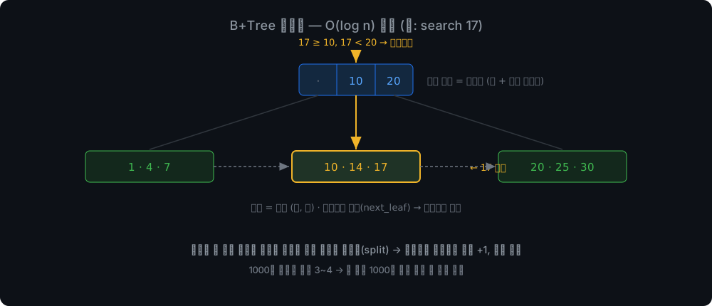
B+Tree는 노드 하나(=페이지 하나)에 키를 수십~수백 개 담아 부채살처럼 갈라집니다(high fan-out, f). 높이가 log₂N이 아니라 log_f N입니다. 같은 100만 행이라도 fan-out이 수백이면 대략 3~4단에 그칩니다(8KB 페이지 기준). “한 번의 디스크 I/O로 가능한 많은 키를 본다”, 이게 B+Tree의 전부입니다.

실무/면접 포인트: 이 “3~4단”은 암산으로 나옵니다. 8KB 페이지에 엔트리(키+포인터) 하나가 수십 바이트면 fan-out은 수백입니다. 300으로 잡으면 300³ ≈ 2,700만, 300⁴ ≈ 81억. 그래서 “수천만~수십억 행도 트리 높이는 3~4”라는 감이 섭니다. 게다가 루트·내부 노드는 거의 항상 버퍼 풀에 상주하니, 점 조회의 실제 디스크 I/O는 리프 근처 1~2번입니다.

구조는 두 종류의 노드로 나뉩니다.

• 내부 노드는 길잡이만 합니다. “키 + 자식 포인터”를 들고 찾는 키를 아래로 내려보냅니다. 실제 값(RID)은 없습니다.
• 리프 노드에는 진짜 “키 → RID”가 여기 있고, 옆 리프와 사슬로 연결돼 있습니다(next_leaf). 이 사슬이 범위 스캔의 핵심입니다(3절).

1
#define BT_MAX_KEYS 8   /* 학습용으로 작게: 분할/다단계가 잘 보이게 */
2

3
typedef struct {
4
    uint8_t  is_leaf;
5
    uint16_t num_keys;
6
    uint64_t next_leaf;            /* 리프 형제 페이지 id. 내부 노드는 미사용 */
7
    bkey_t   keys[BT_MAX_KEYS + 1];
8
    union {
9
        bval_t   values[BT_MAX_KEYS + 1];     /* 리프: 키 -> RID */
10
        uint64_t children[BT_MAX_KEYS + 2];   /* 내부: 자식 페이지 id들 */
11
    } u;
12
} BTNode;

주의: db-hobby는 노드당 키를 8개로 작게 잡았다. 분할이 자주 일어나 눈에 잘 보이게 하려는 학습용 선택이다. 진짜 DB는 페이지를 꽉 채워 수백 개를 담는다. 키가 적든 많든 알고리즘은 한 글자도 안 바뀐다.

2. 가장 어려운 부분: 노드 분할

B+Tree에서 제일 까다로운 게 노드 분할(split) 입니다. 리프가 꽉 차면 반으로 쪼개고 가운데(분리) 키를 부모에게 올립니다. 부모도 꽉 차면 부모가 또 쪼개지고, 루트까지 전파됩니다. 루트가 쪼개질 때만 트리 높이가 1 자랍니다.

여기서 B+Tree가 “균형(Balanced)“을 유지하는 비밀이 나옵니다. AVL처럼 회전으로 맞추는 게 아니라, 위가 아니라 아래(리프)에서 자라기 때문에 모든 리프가 항상 같은 깊이입니다. 한쪽으로 절대 기울지 않습니다.

리프 분할은 뒤 절반을 새 리프로 옮기고, 그 첫 키를 부모로 복사(copy up) 합니다. 리프엔 실제 값이 있으니 키가 양쪽에 남아야 하기 때문입니다.

1
/* 리프 분할: 뒤 절반을 새 리프로 옮기고 첫 키를 위로 복사 */
2
r->next_leaf = n->next_leaf;   /* 새 리프가 사슬을 이어받고 */
3
n->next_leaf = rpid;           /* 옛 리프는 새 리프를 가리킨다 */
4
*sep_out = r->keys[0];         /* 부모로 올라갈 분리 키 (복사) */

내부 노드 분할은 미묘하게 다릅니다. 가운데 키를 복사가 아니라 위로 올려보냅니다(push up). 내부 노드의 키는 길잡이일 뿐이라 양쪽에 둘 필요가 없습니다.

핵심 구분: 리프는 copy up, 내부는 push up. 이 차이가 B+Tree(값은 리프에만, 리프끼리 옆으로 연결)와 B-Tree(값이 내부 노드에도 들어감)를 가르는 지점이기도 하다. PostgreSQL nbtree·InnoDB 모두 B+Tree 계열이다. 더 정확히 말하면 PostgreSQL nbtree는 Lehman-Yao B-link tree로, 모든 노드가 우측 형제로 가는 링크를 하나 더 들고, 분할과 동시 탐색이 겹치는 순간을 이 링크가 구한다. 그 latch 이야기는 8편(병렬 실행)에서 다룬다.

분할 “비율”도 실전 다이얼입니다. db-hobby는 항상 반반으로 쪼개지만, PostgreSQL은 최우측 리프가 차면 90/10으로 쪼갭니다. 단조 증가 키(AUTO_INCREMENT, 타임스탬프)의 삽입은 항상 오른쪽 끝에서만 일어나니, 왼쪽에 반을 남겨봐야 영영 채워지지 않습니다.

실무 안티패턴: 랜덤 UUIDv4를 InnoDB PK로 쓰는 것. InnoDB는 데이터 자체가 PK 순서로 정렬된 클러스터드 구조라, 랜덤 키는 삽입을 트리 전역에 흩뿌려 분할 폭풍과 버퍼 풀 오염(사실상 모든 리프가 워킹셋)을 부릅니다. 대안은 순차성 있는 키, 곧 AUTO_INCREMENT나 시간 정렬 UUIDv7입니다. 힙 vs 클러스터드가 이 비용을 어떻게 가르는지는 7편에서 실측합니다.

디스크에 저장되는 이 트리에 키 1000개를 넣어 다단계 분할을 일으킨 뒤, 리프 사슬을 따라 끝까지 훑어 “정렬이 한 번도 깨지지 않았는지”로 구조 무결성을 검증했습니다. 분할이 루트까지 전파돼도 리프 전체는 여전히 하나의 정렬된 사슬이라는 게 핵심입니다.

3. 범위 스캔: 리프 사슬이 빛나는 순간

WHERE id = 2 같은 점 조회는 루트에서 리프로 내려가 한 줄(O(log n))입니다. 리프 사슬이 빛나는 순간은 범위 스캔입니다. id > 5면 5가 들어갈 리프로 한 번만 내려간 뒤, 거기서부터 next_leaf를 타고 옆으로 끝까지 읽습니다. 트리를 다시 탐색할 필요가 전혀 없습니다.

1
int btree_seek_scan(BTree *bt, bkey_t start, btree_visit_fn visit, void *ctx) {
2
    /* 1) start가 들어갈 리프로 바로 내려간다 (O(log n)) */
3
    /* 2) 그 리프부터 next_leaf 체인을 따라가며 start 미만 키만 건너뛴다 */
4
    while (pid != 0) {
5
        BTNode *n = fetch(bt, pid);
6
        for (int i = 0; i < n->num_keys; i++) {
7
            if (n->keys[i] < start) continue;
8
            visit(n->keys[i], n->u.values[i], ctx);
9
        }
10
        pid = n->next_leaf;   /* 옆 리프로 */
11
    }
12
}

정직한 경계가 하나 있습니다. db-hobby의 리프 사슬은 next_leaf 단방향이라, 역방향 스캔(ORDER BY ... DESC)은 이 구조로 못 받습니다. PostgreSQL의 리프는 양방향 링크라 거꾸로도 훑습니다.

해시 인덱스가 절대 못 하는 게 바로 이겁니다. 해시는 순서를 안 지키니 >도 ORDER BY도 통째로 안 됩니다. SQL은 범위 질의가 너무 흔해서, “점 조회 + 범위 + 정렬”을 한 구조로 다 받는 B+Tree가 기본값이 됐습니다.

흔한 오해 정정: “PostgreSQL 해시 인덱스는 쓰면 안 되는 물건이다?” 이건 10 이전 얘기입니다. 그때는 해시 인덱스가 WAL 로깅이 안 돼 크래시에 유실되고 복제도 안 됐지만, PostgreSQL 10부터는 WAL 로깅되어 크래시에 안전하고 복제도 됩니다. 다만 등호 조회밖에 못 받는 건 구조 그대로라, 범위나 정렬이 하나라도 필요하면 여전히 B-Tree입니다.

LSM은 무작위 쓰기를 순차 쓰기로 바꾸는 정반대 내기인데, 이 갈림길은 7편(저장 엔진의 세 철학)에서 직접 구현해 대조합니다.

4. 유일성을 내려놓으면: 중복 키와 하한 탐색

여기까지의 인덱스는 PK(유일 키) 전용입니다. 그런데 실무에서 인덱스를 거는 컬럼은 대부분 PK가 아닙니다. email, status, created_at 같은, 유일하지 않은 컬럼입니다. “보조 인덱스가 어렵다”의 정체가 바로 이 비유니크성입니다. PK 인덱스가 “유일하다”는 사실에 기대 조용히 넘어가던 가정들이 하나씩 깨집니다.

쓰기는 플래그 하나, 읽기가 진짜 문제

나이 20인 사람이 셋이면 키 20에 RID가 셋 달려야 합니다. 쓰기는 “같은 키면 덮어쓴다”를 “같은 키도 새 항목으로 추가한다”로 바꾸는 플래그 하나로 끝납니다(btree_insert_dup). 진짜 문제는 읽기입니다. 중복 키는 리프 분할 때문에 여러 리프에 흩어집니다.

20이 잔뜩 쌓여 리프가 쪼개지면 분리키가 하필 20이 될 수 있습니다. 그러면 20짜리 항목이 왼쪽 리프에도 오른쪽 리프에도 걸칩니다. 유니크 검색처럼 “분리키와 같으면 오른쪽으로(>=)” 내려가면 왼쪽에 흩어진 20들을 놓칩니다.

그래서 하한 탐색(lower bound) 이 필요합니다. 분리키와 같으면 오른쪽으로 넘어가지 않고(> 비교) 왼쪽 자식으로 내려가, 20이 시작될 수 있는 가장 왼쪽 리프에 닿은 뒤, 리프 사슬을 오른쪽으로 훑으며 20을 다 모으고 21을 만나면 멈춥니다.

1
while (i < n->num_keys && key > n->keys[i]) {  /* '>=' 아니라 '>' */
2
    i++;
3
}

주의: >=를 >로 바꾸는 한 글자가 전부처럼 보이지만, 이게 안 되면 결과가 조용히 일부만 나온다. 에러도 안 나고 그냥 행 몇 개가 빠진다. 인덱스 버그 중 가장 잡기 어려운 종류, 곧 “틀린 결과를 멀쩡한 얼굴로 돌려주는” 버그다. 같은 키 50개를 일부러 여러 리프로 쪼갠 뒤 전부 찾아지는지가 이 코드의 회귀 테스트다.

흔한 오해 정정: “실제 DB도 중복 키를 이렇게 하한 탐색으로 푼다?” 방향이 반대입니다. db-hobby는 유일성을 내려놓고 읽기 쪽(하한 탐색)을 고치는 길을 갔지만, 실제 DB는 유일성을 인공적으로 복원합니다. PostgreSQL은 12부터 모든 인덱스 엔트리에 heap TID를 마지막 정렬 컬럼처럼 붙입니다. nbtree README의 표현 그대로 *“heap TID is treated as a tiebreaker column”*이라, 트리 안의 모든 엔트리가 (키, TID) 조합으로 다시 유일해지고, “같은 키 어디로 내려가지?”라는 문제 자체가 사라집니다. 13부터는 같은 키의 엔트리들을 deduplication으로 압축까지 합니다. InnoDB는 보조 인덱스 키 뒤에 PK를 suffix로 붙여 같은 효과를 냅니다.

참고로 인덱스는 재시작에도 살아남아야 하므로, “이 테이블엔 age_idx가 age 컬럼에 있다”는 정의를 카탈로그에 적고 인덱스 자체는 별도 파일에 둡니다. PostgreSQL이 pg_class/pg_index에 메타데이터를 적고 인덱스를 별도 relation(relfilenode 파일)에 두는 것과 같은 분리입니다.

5. 인덱스는 후보일 뿐: 재검사, 진실은 힙에 있다

보조 인덱스가 준 RID를 곧이곧대로 믿으면 안 됩니다. 이유가 셋입니다.

그래서 후보 RID마다 힙에서 행을 읽고 WHERE를 다시 평가해 진짜 맞는 행만 내보냅니다. 이게 재검사(recheck) 입니다.

핵심: “인덱스는 후보를 좁히고, 진실은 힙에 있다.” 이게 인덱스 스캔의 본질이다. 이 원칙 덕에 B+Tree에 삭제 기능이 없어도, stale 항목이 남아 있어도 결과는 정확하다.

실제 DB와의 대조를 정확히 하면, PostgreSQL의 recheck는 인덱스가 후보만 보장하는 lossy 케이스(GIN/GiST/BRIN, Bitmap Heap Scan)에서 주로 나오고 B-tree 등식 스캔엔 보통 recheck가 없습니다. db-hobby의 재검사는 stale RID(tombstone·슬롯 재사용) 때문이라 이유는 다르지만, “인덱스는 좁히고 최종 판정은 실제 행으로”라는 아이디어는 같습니다.

그리고 이 원칙은 나중에 더 크게 돌아옵니다. 4편(MVCC)에서 UPDATE가 행의 새 버전을 만들기 시작하면, PK 인덱스조차 한 키에 여러 RID(버전들)를 매다는 멀티맵이 됩니다. 인덱스는 버전 후보들을 주고, 어느 버전이 “보이는지”는 힙의 가시성 게이트가 판정합니다. “인덱스는 단순 key→value가 아니다”라는 이 편의 부제가 그 얘기입니다.

6. 플래너의 씨앗: 연산자 하나로 실행 계획이 갈린다

인덱스를 실행기에 연결하면 쿼리 플래너의 씨앗이 생깁니다.

다만 이건 “쓸 수 있으면 무조건 인덱스”라는 규칙 기반(RBO) 의 가장 단순한 형태입니다. 진짜 플래너는 통계로 선택도를 추정해 비용으로 고릅니다. id > 1처럼 대부분 행이 걸리는 조건이면 풀 스캔이 오히려 빠릅니다. 그 얘기는 6편(비용 기반 옵티마이저)에서 규칙이 실제로 틀리는 순간부터 시작합니다.

그리고 인덱스 자체도 공짜가 아닙니다. 인덱스가 하나 늘 때마다 모든 INSERT/UPDATE/DELETE가 그 B+Tree까지 함께 고쳐야 하니, 읽기 한 종류를 빠르게 하려고 쓰기 전부에 세금을 매기는 셈입니다. “일단 다 걸어두자”가 안 되는 이유입니다.

7. 정리

• B+Tree인 이유는 디스크: 노드=페이지, fan-out이 높이를 log_f N으로 무너뜨린다. “한 번의 I/O로 최대한 많은 키를.”
• 분할이 균형의 비밀: 리프에서 위로 자라니 모든 리프가 같은 깊이. 리프는 copy up, 내부는 push up(B+Tree vs B-Tree의 갈림).
• 리프 사슬이 범위 스캔을 공짜로 만든다: 내려가긴 한 번, 나머진 옆으로. 해시가 못 하는 것.
• 유일성을 내려놓으면 하한 탐색이 필요하다: >= 한 글자가 조용히 행을 잃게 만든다.
• 인덱스는 후보일 뿐, 진실은 힙에: 재검사가 stale 항목을 무해화한다. MVCC가 오면 이 원칙이 인덱스의 생존 조건이 된다.
• 실측: 인덱스 vs 풀 스캔 격차는 1천 행 11배 → 10만 행 416배. O(log n)의 가치는 N과 함께 자란다.

다음 편은 쓰기 경로의 대사건입니다. 쓰다가 전원이 꺼지면? WAL과 크래시 복구, 그리고 fsync의 가격(같은 5천 행 적재가 23배 차이 나는 이유)을 다룹니다.

참고 (1차 자료 우선)

• PostgreSQL Documentation: B-Tree Indexes (nbtree)
• PostgreSQL Documentation: Index Access Method Interface
• PostgreSQL Documentation: Hash Indexes
• PostgreSQL source: nbtree README — heap TID tiebreaker · deduplication · Lehman-Yao
• MySQL 8.0 Reference: InnoDB Index Types
• Lehman & Yao, Efficient Locking for Concurrent Operations on B-Trees (ACM TODS, 1981)
• Goetz Graefe, Modern B-Tree Techniques (Foundations and Trends in Databases, 2011)
• 본 블로그: DB 인덱스 ①: 기초와 EXPLAIN · ②: 스캔의 종류 · ③: Covering Index · ④: 복합 인덱스 · ⑤: 클러스터형
• db-hobby 코드 (GitHub) — btree.c

0. Introduction — the O(n) Wall

Part 1 built up to the heap file. Run WHERE id = 2 and a full scan executes — a double loop over every slot of every page. A million rows means a million looks: O(n).

An index turns that into O(log n). The idea is simple — keep a “key → row address (RID)” mapping in a sorted search structure.

Key definition: (in heap-based systems like PostgreSQL and db-hobby) an index is a sorted search structure separate from the data, holding “key → RID.” The heap piles rows unordered; the index lays a sorted road on top for O(log n) lookups. (InnoDB’s clustered index keeps the data itself in the leaves, so the definition shifts — contrasted in Part 7.)

Numbers first. Finding the same single row two ways while growing table size N (C implementation, -O2):

(These numbers are warm-cache — pages resident in the buffer pool. With a cold cache and real disk I/O in the loop, the gap widens further.)

What matters is the shape of the two columns, not the individual numbers. The full-scan column multiplies ~10× every time N does — the shape of O(n). The index column grows just 2.3× while N grows 100× — the log curve of O(log n). So the gap widens as N grows. An index’s value grows with the data — precisely where you need it.

This part builds that index and records what you learn by building it — why a B+Tree, what’s hardest, and what assumptions break the moment you give up uniqueness (secondary indexes).

1. Why a B+Tree, Not a Binary Tree — the Disk Is the Answer

Wouldn’t a binary search tree do? The crux is the disk.

An index also lives on disk in pages. Store a binary tree naively as node = page and, with one key per node, its height is log₂(n) — one page read per level. A million rows ≈ 20 levels ≈ up to 20 page reads (minus buffer-pool hits).

A B+Tree packs dozens to hundreds of keys into one node (= one page), fanning out wide (fan-out f). Height becomes log_f N instead of log₂N — for the same million rows, with fan-out in the hundreds it’s roughly 3–4 levels (8KB pages). “See as many keys as possible per disk I/O” — that’s the whole point of a B+Tree.

Practical/interview point: that “3–4 levels” comes out of mental arithmetic. With an 8KB page and entries (key + pointer) of a few dozen bytes, fan-out lands in the hundreds — take 300: 300³ ≈ 27 million, 300⁴ ≈ 8.1 billion. Hence the intuition “tens of millions to billions of rows, tree height still 3–4.” And since the root and internal nodes are almost always resident in the buffer pool, a point lookup’s real disk I/O is 1–2 reads near the leaf.

Two node kinds:

• Internal nodes — guides only: “key + child pointer,” routing the search downward. No values (RIDs).
• Leaf nodes — the real “key → RID” lives here, and leaves are chained sideways (next_leaf). That chain is the heart of range scans (§3).

1
#define BT_MAX_KEYS 8   /* small on purpose: splits and multi-level growth stay visible */
2

3
typedef struct {
4
    uint8_t  is_leaf;
5
    uint16_t num_keys;
6
    uint64_t next_leaf;            /* leaf sibling page id; unused for internals */
7
    bkey_t   keys[BT_MAX_KEYS + 1];
8
    union {
9
        bval_t   values[BT_MAX_KEYS + 1];     /* leaf: key -> RID */
10
        uint64_t children[BT_MAX_KEYS + 2];   /* internal: child page ids */
11
    } u;
12
} BTNode;

Note: db-hobby caps keys at 8 per node — a learning choice so splits happen often and stay visible. Real DBs pack hundreds per page. The algorithm doesn’t change by a single character either way.

2. The Hardest Part — Node Splits

The trickiest thing in a B+Tree is the split. When a leaf fills, split it in half and promote the middle (separator) key to the parent. If the parent is full, it splits too, propagating up to the root. Only when the root splits does the tree grow taller by one.

Here’s the secret of how a B+Tree stays balanced — not by rotations like AVL, but because it grows from the bottom (leaves), not the top, every leaf is always at the same depth. It can never lean.

A leaf split moves the back half to a new leaf and copies the first key up (leaves hold real values, so the key must remain on both sides):

1
/* leaf split: move the back half to a new leaf; copy its first key up */
2
r->next_leaf = n->next_leaf;   /* new leaf inherits the chain */
3
n->next_leaf = rpid;           /* old leaf points at the new one */
4
*sep_out = r->keys[0];         /* separator key promoted (copied) to the parent */

An internal split differs subtly — the middle key is pushed up, not copied: internal keys are guides only, no need to keep them on both sides.

Key distinction: leaves copy up, internals push up. That difference is also what separates a B+Tree (values only in leaves, leaves chained) from a B-Tree (values in internal nodes too). PostgreSQL’s nbtree and InnoDB are both B+Tree-family. More precisely, PostgreSQL’s nbtree is a Lehman-Yao B-link tree — every node carries one extra link to its right sibling, and that link is what saves the moment a split and a concurrent search collide. The latch story comes in Part 8 (Parallel Execution).

The split ratio is a practical dial too. db-hobby always splits half-and-half, but PostgreSQL splits the rightmost leaf 90/10 — with monotonically increasing keys (AUTO_INCREMENT, timestamps) inserts only ever land at the right end, so leaving half the space on the left would never get filled.

Real-world anti-pattern: using random UUIDv4 as an InnoDB PK. InnoDB is clustered — the data itself is sorted by PK — so random keys scatter inserts across the entire tree, inviting a split storm and buffer pool pollution (effectively every leaf becomes the working set). The alternative is a key with sequential character — AUTO_INCREMENT, or time-ordered UUIDv7. How heap vs clustered splits this cost is measured in Part 7.

Integrity was verified by inserting 1,000 keys to force multi-level splits, then walking the leaf chain end to end checking the ordering never breaks. Even as splits propagate to the root, the leaves remain one sorted chain.

3. Range Scans — Where the Leaf Chain Shines

A point lookup descends root→leaf for one row (O(log n)). The leaf chain shines on range scans: for id > 5, descend once to the leaf where 5 would live, then read sideways along next_leaf to the end — no re-descending, ever.

1
int btree_seek_scan(BTree *bt, bkey_t start, btree_visit_fn visit, void *ctx) {
2
    /* 1) descend straight to the leaf where `start` would live (O(log n)) */
3
    /* 2) from there, follow the next_leaf chain, skipping keys < start */
4
    while (pid != 0) {
5
        BTNode *n = fetch(bt, pid);
6
        for (int i = 0; i < n->num_keys; i++) {
7
            if (n->keys[i] < start) continue;
8
            visit(n->keys[i], n->u.values[i], ctx);
9
        }
10
        pid = n->next_leaf;   /* sideways */
11
    }
12
}

One honest boundary — db-hobby’s leaf chain is one-directional (next_leaf), so backward scans (ORDER BY ... DESC) can’t ride this structure. PostgreSQL’s leaves are doubly linked and sweep both ways.

This is exactly what a hash index can never do — hashes keep no order, so > and ORDER BY are impossible wholesale. SQL is so full of range queries that the B+Tree — point + range + order in one structure — became the default.

Common misconception, corrected: “PostgreSQL hash indexes are a forbidden feature?” — That’s pre-10 lore. Back then hash indexes weren’t WAL-logged, so they were lost on crash and never replicated; since PostgreSQL 10 they are WAL-logged, crash-safe, and replicable. The structural limit stands, though — equality lookups only — so the moment you need any range or ordering, it’s still the B-Tree.

The LSM is the opposite bet — turning random writes into sequential ones — built and contrasted head-on in Part 7.

4. Giving Up Uniqueness — Duplicate Keys and Lower-Bound Search

So far the index served the PK (unique keys). But in practice most indexed columns aren’t PKs — they’re email, status, created_at: not unique. That’s the real identity of “secondary indexes are hard.” Assumptions the PK index quietly leaned on break one by one:

Writes Are One Flag; Reads Are the Real Problem

If three people are age 20, key 20 must carry three RIDs. Writing is a one-flag change (“same key overwrites” → “same key appends,” btree_insert_dup). The real problem is reading. Duplicate keys get scattered across leaves by splits.

Pile up enough 20s and a leaf splits with the separator key happening to be 20 — now 20-entries straddle both the left and right leaf. Descend like the unique search does (“if equal to separator, go right,” >=) and you miss the 20s on the left.

Hence lower-bound search: when equal to a separator, do not go right (> comparison, not >=) — descend left to reach the leftmost leaf where 20 could start, then sweep the leaf chain rightward collecting 20s until a 21 appears.

1
while (i < n->num_keys && key > n->keys[i]) {  /* '>' — not '>=' */
2
    i++;
3
}

Warning: changing >= to > looks like one character, but without it results come back silently partial. No error — just missing rows. The hardest class of index bug: one that returns wrong results with a straight face. The regression test plants 50 identical keys deliberately split across leaves and asserts all 50 are found.

Common misconception, corrected: “real DBs also solve duplicate keys with lower-bound search?” — The direction is reversed. db-hobby gives up uniqueness and fixes the read side (lower-bound search); real DBs artificially restore uniqueness. Since version 12, PostgreSQL appends the heap TID to every index entry as if it were a trailing sort column — in the nbtree README’s own words, “heap TID is treated as a tiebreaker column” — so every entry in the tree is unique again as a (key, TID) pair, and the question “which way down for equal keys?” simply disappears. Since 13, entries with equal keys are further compressed by deduplication. InnoDB gets the same effect by suffixing the PK onto secondary index keys.

Since indexes must also survive restarts, the definition (“table t has age_idx on column age”) goes into the catalog and the index lives in its own file — the same separation as PostgreSQL recording metadata in pg_class/pg_index while the index lives in its own relation (relfilenode) file.

5. The Index Only Narrows — Recheck; the Truth Lives in the Heap

You must not take a secondary index’s RIDs at face value. Three reasons:

So for each candidate RID, read the row from the heap and re-evaluate WHERE, emitting only true matches. That’s the recheck.

Key principle: “the index narrows candidates; the truth lives in the heap.” That’s the essence of an index scan. Thanks to it, results stay correct even with no B+Tree delete and with stale entries lying around.

To be precise about the real-DB contrast: PostgreSQL’s recheck appears mainly where the index is lossy (GIN/GiST/BRIN, Bitmap Heap Scan); plain B-tree equality scans usually need none. db-hobby’s recheck exists because of stale RIDs (tombstones, slot reuse) — different reason, same idea: the index narrows, the actual row decides.

And this principle returns in a bigger way: in Part 4 (MVCC), once UPDATE starts creating new row versions, even the PK index becomes a multimap hanging several RIDs (versions) off one key — the index yields version candidates, and the heap’s visibility gate decides which one is “visible.” That’s what this part’s subtitle — “why an index isn’t a simple key→value map” — is about.

6. The Seed of a Planner — One Operator Changes the Plan

Wiring the index into the executor plants the seed of a query planner:

But this is the crudest rule-based (RBO) form: “use an index whenever possible.” A real planner estimates selectivity from statistics and chooses by cost — for a condition like id > 1 matching most rows, a full scan is actually faster. That story starts in Part 6 (Cost-Based Optimizer), at the exact moment the rule goes wrong.

And indexes themselves aren’t free — every additional index means every INSERT/UPDATE/DELETE must also maintain that B+Tree. To speed up one kind of read, you’re taxing every write. That’s why “just index everything” doesn’t work.

7. Wrap-up

• The reason it’s a B+Tree is the disk — node = page; fan-out collapses height to log_f N. “As many keys per I/O as possible.”
• Splits are the secret of balance — growing upward from the leaves keeps all leaves at equal depth. Leaves copy up, internals push up (the B+Tree vs B-Tree fork).
• The leaf chain makes range scans free — descend once, go sideways. What hashes can’t do.
• Give up uniqueness and you need lower-bound search — one >= silently loses rows.
• The index only narrows; the truth lives in the heap — recheck neutralizes stale entries. Under MVCC this principle becomes the index’s survival condition.
• Measured: index vs full scan widens from 11× (1k rows) to 416× (100k). O(log n)‘s value grows with N.

Next: the write path’s great event — what if the power dies mid-write? WAL and crash recovery, and the price of fsync (why loading the same 5,000 rows differs by 23×).

References (primary sources first)

• PostgreSQL Documentation: B-Tree Indexes (nbtree)
• PostgreSQL Documentation: Index Access Method Interface
• PostgreSQL Documentation: Hash Indexes
• PostgreSQL source: nbtree README — heap TID tiebreaker · deduplication · Lehman-Yao
• MySQL 8.0 Reference: InnoDB Index Types
• Lehman & Yao, Efficient Locking for Concurrent Operations on B-Trees (ACM TODS, 1981)
• Goetz Graefe, Modern B-Tree Techniques (Foundations and Trends in Databases, 2011)
• This blog: DB Index ①–⑤
• db-hobby source (GitHub) — btree.c