모든 글
약 20분 분량 학습 프로젝트/토이 DB

DB 내부 ⑦: 저장 엔진의 세 철학: 힙 vs 클러스터드 vs LSM, 그리고 USING lsm
목차

0. 들어가며: 같은 행, 세 가지 저장 철학

지금까지의 엔진은 1편에서 고른 (PostgreSQL식) 위에 서 있습니다. 그런데 그건 세 철학 중 하나일 뿐입니다.

철학대표한 줄 요약
PostgreSQL순서 없이 쌓고, 인덱스가 RID(물리 위치)로 가리킨다
클러스터드MySQL InnoDB데이터 자체를 PK 순서로 정렬해 저장한다
LSMRocksDB·Cassandra제자리에서 절대 안 고친다. 쓰기는 전부 append

교과서는 이 셋의 장단점을 문장으로 말합니다. “클러스터드는 PK 범위에 유리하다”, “LSM은 쓰기에 유리하다”. 이 편은 한 코드베이스에 셋을 다 세워 그 문장들을 숫자로 만듭니다. 그리고 마지막엔 LSM을 진짜 엔진에 CREATE TABLE ... USING lsm으로 배선하며 부딪힌, 교과서에 잘 안 나오는 벽까지.

1. 힙 vs 클러스터드: 두 거인의 정반대 선택

구조 차이부터. 에선 행이 아무 데나 살고, PK 인덱스가 “키 → RID”(PostgreSQL 용어로는 TID, ctid로 노출되는 그것)로 가리킵니다(조회 = 인덱스 하강 + 힙 페치, 2단계). 클러스터드에선 PK 인덱스의 리프가 곧 데이터입니다(조회 = 트리 하강 한 번). 대신 보조 인덱스가 갈립니다. 힙의 보조 인덱스는 RID를 들지만, 클러스터드의 보조 인덱스는 PK 값을 들고 “보조 트리 → PK 트리 → 데이터”의 이중 조회를 합니다(행이 페이지 분할로 옮겨 다니니 물리 포인터를 들 수 없기 때문입니다).

같은 데이터를 두 구조로 만들어 실측하면(동일 비용 모델·동일 머신):

접근 경로힙 (PG식)클러스터드 (InnoDB식)결과
PK 점 조회인덱스→RID→힙트리 하강 한 번클러스터드 1.2배 빠름
PK 범위 스캔RID마다 힙 페치(흩어짐)리프가 데이터라 순서대로 쭉클러스터드 3.8배 빠름
보조 점 조회보조→RID→힙보조→PK 트리 또 하강→데이터클러스터드 2배 느림

방향이 교과서 문장과 맞아떨어집니다. 크기(1.2배·3.8배·2배)는 일반 상수가 아니라 행 폭과 캐시 상주 여부에 따라 달라지는 값입니다. 이 측정은 warm(메모리 상주) 기준이고, 콜드 디스크에선 지역성 이득이 수십 배로 벌어질 수 있습니다.

  • PK 범위 3.8배: 클러스터드의 본질인 지역성입니다. PK 순서로 정렬돼 있으니 범위 스캔이 연속 페이지를 쭉 읽습니다. 힙은 RID들이 흩어진 페이지를 하나씩 페치합니다.
  • 보조 2배 열세: InnoDB의 유명한 이중 조회(double lookup) 비용이 그대로 재현됩니다. MySQL 매뉴얼의 문장 그대로입니다. “each secondary index record contains the primary key columns”: 보조 인덱스가 물리 포인터 대신 PK 값을 들고 있으니, 데이터까지 가려면 PK 트리를 한 번 더 내려갑니다.

물론 실제 DB들은 이 비용을 그냥 두지 않습니다. InnoDB에선 보조 인덱스에 PK 컬럼이 공짜로 들어가니, 자주 읽는 컬럼까지 담은 커버링 인덱스로 짜면 PK 트리 하강 자체를 생략할 수 있습니다. PostgreSQL 쪽의 힙 페치도 index-only scan으로 건너뛸 수 있습니다. 단, 후자는 visibility map이 “이 페이지는 전부 가시”라고 보증할 때만 성립해서, VACUUM이 밀리면 도로 힙을 찾아갑니다.

핵심: “어느 쪽이 더 좋다”가 아니라 “무엇에 최적화됐나” 다. PK 중심의 조회·범위가 많으면 클러스터드(InnoDB), 쓰기가 단순하고 보조 인덱스가 많으면 힙(PG)이 유리하다. 워크로드가 답을 정한다. 이론은 DB 인덱스 ⑤: 클러스터형 인덱스와 DBMS별 차이.

“힙이냐 클러스터드냐”의 선택권도 DB마다 다릅니다:

DBMS기본 테이블 조직비고
PostgreSQL힙 전용tableam API로 다른 조직을 꽂을 수는 있음
MySQL InnoDB클러스터드 강제PK가 없으면 내부적으로 GEN_CLUST_INDEX를 만들어서라도 클러스터링
SQL Server힙/클러스터드 선택클러스터드 인덱스를 두는 게 사실상 관례
Oracle힙 기본IOT(Index-Organized Table) 옵션으로 클러스터드형 조직 선택 가능

실무 안티패턴: InnoDB 테이블에 UUIDv4를 PK로 쓰는 것. 클러스터드는 데이터 자체가 PK 순서라, 무작위 PK는 삽입마다 트리의 무작위 지점을 두드려 페이지 분할을 전역으로 일으킵니다(버퍼 풀 오염 + 쓰기 증폭). AUTO_INCREMENT나 시간 정렬 UUIDv7이 대안입니다. 같은 UUIDv4라도 힙(PostgreSQL)에선 행 배치가 PK와 무관해 충격이 훨씬 작습니다.

2. LSM: 제자리에서 절대 안 고친다

세 번째 철학은 더 급진적입니다. B+Tree(힙이든 클러스터드든)는 제자리 갱신(in-place) 입니다. 키가 갈 페이지를 찾아가 그 페이지를 고칩니다. 읽기엔 좋지만, in-place 구조는 결국 흩어진 페이지들의 랜덤 쓰기를 디스크에 반영해야 하고(버퍼 풀과 체크포인트가 이를 지연·병합해 주지만 없애 주진 않습니다) 페이지 분할 비용도 따라옵니다. LSM은 그 랜덤 쓰기마저 순차화하겠다는 발상입니다.

LSM(Log-Structured Merge tree) 은 정반대 내기를 겁니다: 절대 제자리에서 안 고친다.

  1. 모든 쓰기는 인메모리 정렬 구조(memtable)에 append되고,
  2. 임계치를 넘으면 통째로 정렬된 불변 파일(SSTable) 로 순차 flush되고,
  3. 나중에 background로 여러 SSTable을 merge(compaction)해 정리한다.

삭제조차 제자리 삭제가 아니라 tombstone(묘비 마커)을 새로 씁니다. 4편의 MVCC DELETE(xmax 논리 삭제)와 VACUUM(나중에 청소)이 했던 그 지연 삭제와 똑같은 발상입니다.
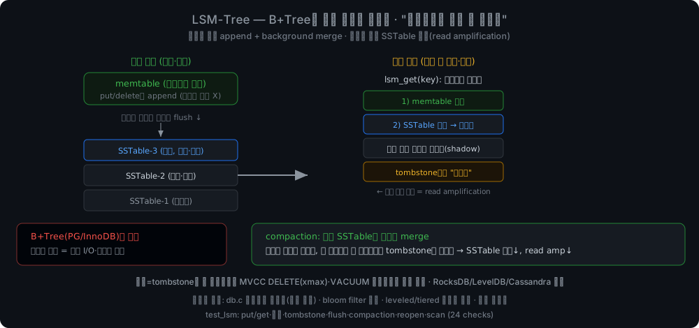
LSM-Tree: memtable append → SSTable 순차 flush → compaction merge. 읽기는 memtable→최신 SSTable 순(read amplification)

대가는 읽기입니다. 한 키를 찾으려면 memtable → 최신 SSTable → … → 가장 오래된 SSTable 순으로 뒤져야 합니다(read amplification). 최신이 옛것을 “가리고(shadow)”, 처음 만난 버전(tombstone 포함)이 이깁니다. RocksDB가 Bloom 필터(확률적 자료구조라 없는 키를 높은 확률로 거름, 키당 10비트 기준 거짓 양성 ~1%, 거짓 음성은 없음)와 compaction 전략으로 이 비용을 깎는 게 LSM 엔지니어링의 절반입니다. compaction도 한 종류가 아닙니다. RocksDB는 leveled(기본)·universal(tiered 계열)·FIFO를 제공하고, 이 선택이 read/write/space amplification의 3자 트레이드오프를 정합니다.

그리고 compaction은 공짜가 아닙니다. 같은 데이터를 여러 번 다시 쓰는 작업이라, 유입 쓰기 1바이트가 디스크엔 그 몇 배로 기록됩니다(write amplification). RocksDB Tuning Guide가 말하는 leveled compaction의 write amp가 보통 10~30배 수준입니다. 그래서 LSM 설계는 read/write/space amplification 세 축의 트레이드오프로 정리됩니다. 셋을 동시에 최적화할 수 없다는 게 RUM 추측(RUM Conjecture)입니다. compaction 전략을 고르는 건 이 삼각형 위에 좌표를 찍는 일입니다.

흔한 오해 정정: “LSM은 쓰기가 빠르다 = 쓰기량이 적다?”. LSM의 이점은 무작위 쓰기를 순차 쓰기로 바꾸는 것이지 총량을 줄이는 게 아닙니다. compaction의 재쓰기까지 합치면 총 디스크 쓰기 바이트는 오히려 B+Tree보다 많을 수 있습니다. “쓰기에 유리하다”의 정확한 의미는 “쓰기 경로가 순차 I/O로 정렬되고, 삽입 처리량과 지연이 안정적”이라는 것.

B+Tree (제자리)LSM (append)
쓰기랜덤 I/O + 분할순차 쓰기 (memtable→flush)
읽기O(log n) 한 트리여러 run 탐색 (read amp)
삭제제자리tombstone (지연)
대표PostgreSQL·InnoDBRocksDB·Cassandra·LevelDB
적합읽기·쓰기 균형 + 트랜잭션쓰기 폭주·로그성

C 구현(memtable = 정렬 배열, 모든 SSTable을 하나로 합치는 full compaction으로 위 스펙트럼에선 사실상 tiered의 극단에 찍히는 좌표, 재오픈 시 *.sst 발견)으로 이 성질들을 전부 테스트로 못박았습니다. flush 경계를 넘은 갱신에서 최신이 가리는지, tombstone이 옛 SSTable 값을 가리는지, compaction 후 살아있는 키가 전부 정확한지, 재오픈 후 flush된 데이터가 생존하는지.

3. 캡스톤: LSM을 진짜 PK 인덱스로 (USING lsm)

여기까지의 LSM은 독립 모듈입니다. MySQL의 MyRocks가 테이블 단위로 저장 엔진을 고르게 하듯, 이걸 진짜 엔진에 꽂아 봅니다. 목표는:

CREATE TABLE t (id INT, v INT) USING lsm;

테이블마다 PK 인덱스 저장 엔진을 B+Tree(읽기 최적)와 LSM(쓰기 최적) 중에 고르는 겁니다. 어디에 꽂을지 봅시다. LSM의 네이티브 API는 int64 → int64인데, PK 인덱스가 정확히 PK(int64) → RID(int64) 입니다. 행 heap은 안 건드리고 PK 인덱스만 교체 가능(pluggable) 하게 만들면 됩니다. 실행기가 인덱스를 만지는 지점들을 작은 추상화(pidx_*)로 라우팅하는, PostgreSQL tableam/MySQL handler API의 축소판입니다.

다만 MyRocks와 겹치는 층은 정확히 이 테이블 단위 pluggable 엔진 API까지입니다. MyRocks는 행 전체를 RocksDB 안에 저장합니다. PK를 키로 인코딩해 나머지 컬럼을 값에 담고, 보조 인덱스는 (인덱스 컬럼+PK)를 키로 한 또 하나의 키 공간입니다. 행 heap은 그대로 두고 PK 인덱스만 갈아 끼우는 내 방식과는 데이터 배치가 다릅니다.

부딪힌 벽: 인덱스는 단순 key→value가 아니다

그런데 막상 꽂으려니 벽이 나왔습니다. 4편에서 본 그것입니다. MVCC 때문에 PK 인덱스는 한 키에 여러 RID(버전들)를 매다는 비유니크 멀티맵입니다. UPDATE가 옛 버전을 남기고 새 버전을 추가하기 때문입니다. 그런데 LSM은 unique(키당 값 하나, 최신이 가림)였습니다. PK=9 → {RID_old, RID_new}를 담을 수 없습니다.

그래서 LSM 자체를 확장했습니다. 멀티값 모드입니다. dedup 단위를 key에서 (key, val) 짝으로 바꿉니다.

int lsm_put_dup(LSM *l, int64_t key, int64_t val); /* (key,val) 짝 추가 — 다른 val 안 가림 */
int lsm_delete_val(LSM *l, int64_t key, int64_t val); /* 그 짝만 tombstone */
int64_t lsm_find_all(LSM *l, int64_t key, cb, ctx); /* key의 살아있는 모든 val */

memtable은 (key, val)로 정렬하고, merge는 (key asc, val asc, 최신도 desc)로 정렬해 짝마다 최신 하나를 채택합니다. 같은 키의 서로 다른 RID가 공존하고, 특정 짝만 지울 수 있습니다. RocksDB 계열이 비유니크 보조 인덱스를 담는 방식과 같은 계열입니다.
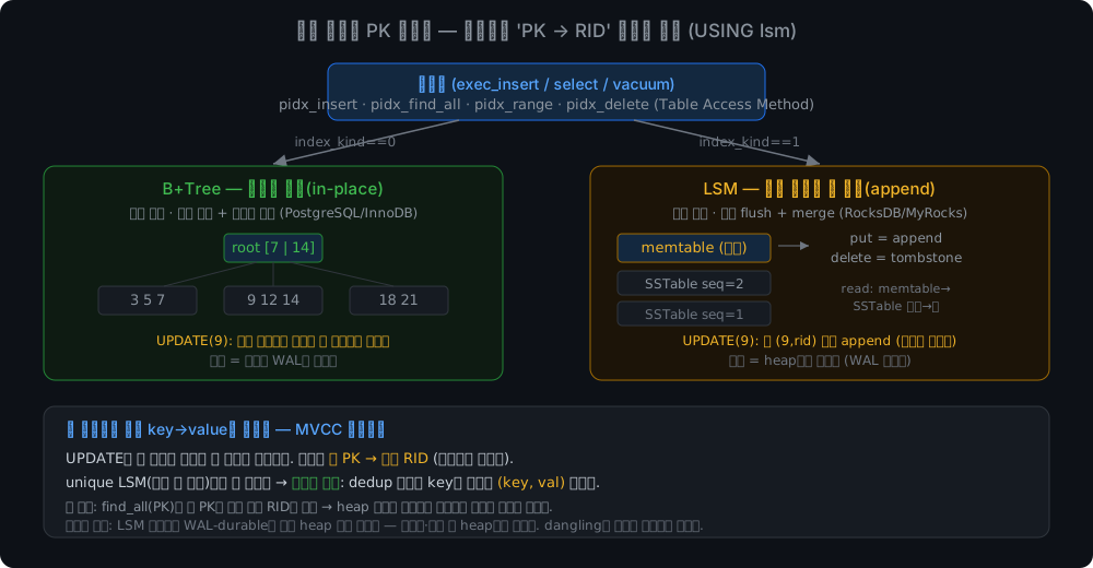
교체 가능한 PK 인덱스: 실행기는 PK→RID 매핑만 알고, pidx가 B+Tree/LSM으로 라우팅한다. MVCC 멀티버전이 멀티값 모드를 강제한다

두 번째 벽: 트랜잭션 롤백에 못 낀다

B+Tree PK 인덱스는 자체 WAL로 트랜잭션 롤백에 참여합니다. 그런데 내 미니 LSM은 자체 WAL이 없어서 그 롤백 기계에 못 낍니다. memtable은 휘발성이고, SSTable은 이미 flush된 append-only 파일이기 때문입니다. 해법은 관점 전환이었습니다:

LSM PK 인덱스는 “권위 있는 진실”이 아니라 heap 위의 파생 가속기다. 읽기 경로가 어차피 인덱스 후보를 heap에서 재검사하므로(2편의 recheck + 4편의 가시성 게이트), 인덱스가 잠깐 부정확해도 결과는 옳다. 그래서 재오픈·롤백 시 heap에서 통째로 재구축하면 되고, 중단된 트랜잭션이 남긴 dangling 항목은 가시성 게이트가 무해화한다.

흔한 오해 정정: “LSM은 트랜잭션이 안 된다?”. 위 제약은 어디까지나 자체 WAL이 없는 내 미니 LSM의 사정이지, LSM 일반의 성질이 아닙니다. 실제 RocksDB는 memtable을 자체 WAL로 보호하고, WriteBatch 위에 pessimistic/optimistic 트랜잭션까지 지원합니다. 그래서 MyRocks에선 롤백이 정상 동작합니다. 덧붙여 “heap에서 재구축되는 파생 가속기”라는 위 설계도 MyRocks의 실제 방식은 아닙니다. MyRocks에선 RocksDB가 heap 옆의 가속기가 아니라 권위 저장소 그 자체이기 때문입니다.

검증은 동치성으로 합니다. USING lsm 테이블과 B+Tree 테이블에 같은 SQL을 던져 점/범위 조회, MVCC UPDATE 가시성, DELETE/VACUUM, ROLLBACK, 재오픈까지 결과가 같은지 확인합니다. 전부 통과했습니다.

4. 정리

  • 세 철학: 힙(순서 없음+RID), 클러스터드(데이터=PK 트리 리프), LSM(절대 제자리 안 고침). “더 좋다”가 아니라 “무엇에 최적화됐나”.
  • 실측: 클러스터드가 PK 점 1.2배·범위 3.8배(지역성) 우세, 보조 점 조회는 2배 열세(이중 조회). 교과서 문장의 방향이 숫자로 확인됐다(크기는 행 폭·캐시 상주에 따라 달라진다).
  • LSM의 내기: 무작위 쓰기를 순차로 바꾸는 대신 read amplification을 지고, compaction의 write amplification도 낸다. 총 쓰기량이 준다는 뜻이 아니다. tombstone은 MVCC의 지연 삭제와 같은 발상.
  • USING lsm 배선의 교훈: ① MVCC 멀티버전이 인덱스를 비유니크 멀티맵으로 강제한다. unique LSM엔 멀티값 모드((key,val) dedup)가 필요했다. ② 자체 WAL이 없어 롤백에 못 끼는 구조는 heap에서 재구축되는 파생 가속기로 다루면 된다. recheck·가시성 게이트가 최종 방어선이니까.

실무/면접 포인트: 저장 엔진 비교의 뼈대는 두 문장입니다. ① 클러스터드는 PK 지역성 덕에 범위 스캔에 유리하지만, 보조 인덱스는 PK 경유 이중 조회 비용을 진다. ② LSM의 “쓰기 유리”는 무작위 쓰기의 순차화지 총량 감소가 아니다. compaction의 write amplification까지 짚으면 답이 한 단계 깊어진다.

다음 편은 이 엔진을 여러 코어로 돌립니다. latch를 계층별로 걷어내는 병렬 실행의 여정(그리고 실측이 알려준 진짜 천장)입니다.

참고 (1차 자료 우선)

0. Introduction — Same Rows, Three Storage Philosophies

The engine so far stands on the heap (PostgreSQL-style) chosen in Part 1. But that’s one philosophy of three:

PhilosophyRepresentativeOne line
HeapPostgreSQLpile unordered; indexes point by RID (physical location)
ClusteredMySQL InnoDBstore the data itself sorted by PK
LSMRocksDB · Cassandranever modify in place — every write is an append

Textbooks state the trade-offs in prose — “clustered favors PK ranges,” “LSM favors writes.” This part stands all three in one codebase and turns those sentences into numbers — then finishes by wiring the LSM into the real engine via CREATE TABLE ... USING lsm, hitting a wall textbooks rarely mention.

1. Heap vs Clustered — Two Giants’ Opposite Choices

Structure first. In a heap, rows live anywhere and the PK index points “key → RID” (PostgreSQL calls this the TID, exposed as ctid) — lookup = index descent + heap fetch: 2 steps. In a clustered table, the PK index’s leaves are the data (lookup = one tree descent). The fork moves to secondary indexes — a heap’s secondaries carry RIDs, but a clustered table’s secondaries carry PK values and pay a double lookup: secondary tree → PK tree → data (rows migrate during page splits, so physical pointers can’t be stored).

Building the same data both ways and measuring (same cost model, same machine):

Access pathHeap (PG-style)Clustered (InnoDB-style)Result
PK point lookupindex→RID→heapone tree descentclustered 1.2× faster
PK range scanheap fetch per RID (scattered)leaves are the data — read straightclustered 3.8× faster
Secondary point lookupsecondary→RID→heapsecondary→descend PK tree again→dataclustered 2× slower

The direction lands on the textbook prose. The magnitudes (1.2×, 3.8×, 2×) are not universal constants — they shift with row width and cache residency. These measurements are warm (memory-resident); on cold disk the locality advantage can widen to tens of times.

  • 3.8× on PK ranges — clustering’s essence, locality: sorted by PK, a range scan reads consecutive pages; the heap fetches scattered pages one by one.
  • 2× behind on secondaries — InnoDB’s famous double lookup, reproduced. In the MySQL manual’s own words — “each secondary index record contains the primary key columns”: the secondary carries PK values instead of physical pointers, so reaching the data means descending the PK tree once more.

Of course, real DBs don’t just eat this cost. In InnoDB the PK columns ride in every secondary for free, so a covering index holding the frequently-read columns skips the PK-tree descent entirely. On the PostgreSQL side the heap fetch can be skipped with an index-only scan — but only when the visibility map vouches that “every row on this page is visible,” so a lagging VACUUM sends you back to the heap.

Key point: not “which is better” but “optimized for what.” PK-centric lookups and ranges favor clustered (InnoDB); simple writes and many secondaries favor the heap (PG). The workload decides. Theory: DB Index ⑤: Clustered Indexes Across DBMSs.

How much choice you get between heap and clustered also varies by DB:

DBMSDefault table organizationNotes
PostgreSQLHeap onlyother organizations pluggable via the tableam API
MySQL InnoDBClustered, mandatorywithout a PK it clusters anyway, on an internal GEN_CLUST_INDEX
SQL ServerHeap or clustered, your choicea clustered index is the de-facto convention
OracleHeap by defaultIOT (Index-Organized Table) as the clustered-style option

Anti-pattern in practice: a UUIDv4 primary key on an InnoDB table. Clustered means the data itself is in PK order, so random PKs hammer random spots in the tree on every insert, causing page splits everywhere (buffer-pool pollution + write amplification). AUTO_INCREMENT or time-ordered UUIDv7 are the alternatives. The same UUIDv4 hurts far less on a heap (PostgreSQL), where row placement is unrelated to the PK.

2. The LSM — Never Modify In Place

The third philosophy is more radical. A B+Tree (heap or clustered) does in-place updates — find the page a key belongs to and modify it. Great for reads; but an in-place structure must eventually push random page writes to disk (the buffer pool and checkpoints defer and coalesce them, but never eliminate them), with page-split costs on top. The LSM’s idea is to sequentialize even those random writes.

The LSM (Log-Structured Merge tree) makes the opposite bet: never modify in place.

  1. Every write appends to an in-memory sorted structure (the memtable);
  2. past a threshold, it’s flushed wholesale into a sorted immutable file (SSTable) — sequentially;
  3. later, background compaction merges SSTables to tidy up.

Even deletion isn’t in-place — it writes a tombstone marker. The same deferred-deletion idea as Part 4’s MVCC DELETE (logical xmax) and VACUUM (clean later).

LSM-Tree — memtable appends → sequential SSTable flushes → compaction merges. Reads search memtable → newest SSTables (read amplification)

The price is reads: finding one key means searching memtable → newest SSTable → … → oldest (read amplification). Newer shadows older; the first version found (including tombstones) wins. Half of LSM engineering — RocksDB’s Bloom filters (a probabilistic structure that rejects absent keys with high probability — ~1% false positives at 10 bits/key, no false negatives) and its compaction strategies — exists to trim this cost. And compaction isn’t one thing: RocksDB offers leveled (the default), universal (tiered-family), and FIFO, and that choice sets the three-way trade-off between read, write, and space amplification.

Compaction isn’t free either — it rewrites the same data multiple times, so one incoming byte lands on disk several times over (write amplification). The RocksDB Tuning Guide puts leveled compaction’s write amp at typically 10–30×. That’s why LSM design boils down to the three-axis trade-off of read/write/space amplification — the RUM Conjecture says you can’t optimize all three at once — and picking a compaction strategy is picking your coordinates on that triangle.

Common misconception, corrected: “LSM writes are fast = LSM writes less?” — the LSM’s advantage is turning random writes into sequential ones, not reducing the total. Counting compaction’s rewrites, total disk bytes written can actually exceed a B+Tree’s. The precise meaning of “write-friendly” is “the write path is aligned into sequential I/O, with stable insert throughput and latency.”

B+Tree (in-place)LSM (append)
Writesrandom I/O + splitssequential (memtable→flush)
ReadsO(log n), one treemultiple runs (read amp)
Deletesin placetombstones (deferred)
RepresentativesPostgreSQL · InnoDBRocksDB · Cassandra · LevelDB
Fitsbalanced R/W + transactionswrite-heavy, log-like

A C implementation (memtable = sorted array; a full compaction merging every SSTable into one — on the spectrum above, effectively the extreme end of tiered; *.sst discovery on reopen) pins all these properties with tests — newest shadowing across a flush boundary, tombstones shadowing old SSTable values, correctness of all live keys after compaction, survival of flushed data across reopen.

3. The Capstone — LSM as the Real PK Index (USING lsm)

So far the LSM is standalone. Like MySQL’s MyRocks letting you pick a storage engine per table, we now plug it into the real engine:

CREATE TABLE t (id INT, v INT) USING lsm;

Each table picks its PK-index storage engine: B+Tree (read-optimized) or LSM (write-optimized). Where does it plug in? The LSM’s native API is int64 → int64, and the PK index is exactly PK(int64) → RID(int64). Leave the row heap alone and make just the PK index pluggable — routing the executor’s index touch-points through a small abstraction (pidx_*), a miniature of PostgreSQL’s tableam / MySQL’s handler API.

To be precise, that table-level pluggable engine API is exactly where the overlap with MyRocks ends. MyRocks stores entire rows inside RocksDB — the PK encoded as the key with the remaining columns in the value, and each secondary index as another key space keyed on (index columns + PK). My approach — leave the row heap alone and swap only the PK index — lays the data out differently.

The Wall — an Index Is Not a Simple key→value Map

Then the wall: as Part 4 showed, MVCC makes the PK index a non-unique multimap hanging several RIDs (versions) off one key — UPDATE leaves the old version and adds a new one. But the LSM was unique (one value per key; newest shadows). It cannot hold PK=9 → {RID_old, RID_new}.

So the LSM itself was extended — a multi-value mode: the dedup unit changes from the key to the (key, val) pair.

int lsm_put_dup(LSM *l, int64_t key, int64_t val); /* add a (key,val) pair — doesn't shadow other vals */
int lsm_delete_val(LSM *l, int64_t key, int64_t val); /* tombstone that pair only */
int64_t lsm_find_all(LSM *l, int64_t key, cb, ctx); /* all live vals for a key */

The memtable sorts by (key, val); merges sort (key asc, val asc, recency desc) and keep the newest per pair. Different RIDs of the same key coexist, and a specific pair can be deleted — the same lineage as how RocksDB-family engines hold non-unique secondary indexes.

Pluggable PK index — the executor knows only the PK→RID mapping; pidx routes to B+Tree or LSM. MVCC multi-versioning forces the multi-value mode

The Second Wall — It Can’t Join Transaction Rollback

The B+Tree PK index participates in rollback via its own WAL. But my mini LSM has no WAL of its own, so it can’t join that machinery — the memtable is volatile and the SSTables are already-flushed append-only files. The fix was a change of perspective:

The LSM PK index is not “authoritative truth” but a derived accelerator over the heap. Since the read path rechecks index candidates against the heap anyway (Part 2’s recheck + Part 4’s visibility gate), the index may be briefly inaccurate without the results ever being wrong. So on reopen/rollback it’s rebuilt wholesale from the heap, and dangling entries from aborted transactions are neutralized by the visibility gate.

Common misconception, corrected: “LSMs can’t do transactions?” — the constraint above is strictly my mini LSM’s lack of a WAL, not a property of LSMs. Real RocksDB protects its memtable with its own WAL and supports pessimistic/optimistic transactions on top of WriteBatch — which is why rollback works fine in MyRocks. And note the “derived accelerator rebuilt from the heap” design above isn’t how MyRocks actually works either — in MyRocks, RocksDB is not an accelerator beside a heap but the authoritative store itself.

Verification by equivalence — the same SQL against a USING lsm table and a B+Tree table must match across point/range lookups, MVCC UPDATE visibility, DELETE/VACUUM, ROLLBACK, and reopen. All green.

4. Wrap-up

  • Three philosophies: heap (unordered + RID), clustered (data = PK tree leaves), LSM (never in place). Not “better” — “optimized for what.”
  • Measured: clustered wins PK point 1.2× and range 3.8× (locality), loses secondary lookups 2× (double lookup). The textbook prose’s direction was confirmed in numbers (magnitudes shift with row width and cache residency).
  • The LSM’s bet: turn random writes sequential, pay read amplification — and compaction’s write amplification too; it never meant writing fewer total bytes. Tombstones are MVCC’s deferred deletion in another coat.
  • Lessons from wiring USING lsm: ① MVCC multi-versioning forces the index to be a non-unique multimap — the unique LSM needed a multi-value mode ((key,val) dedup). ② A structure that can’t join rollback for lack of its own WAL can be treated as a derived accelerator rebuilt from the heap — recheck and the visibility gate are the last line of defense.

Practice/interview point: the skeleton of any storage-engine comparison is two sentences. ① Clustered wins range scans through PK locality, but secondaries pay the double lookup through the PK. ② The LSM’s “write advantage” is the sequentialization of random writes, not a reduction in total volume — mentioning compaction’s write amplification takes the answer one level deeper.

Next: this engine on many cores — the journey of peeling latches off layer by layer for parallel execution, and the real ceiling the measurements revealed.

References (primary sources first)

Author
작성자 @범수

오늘의 노력이 내일의 전문성을 만든다고 믿습니다.

댓글

댓글 수정/삭제는 GitHub Discussions에서 가능합니다.