DB 내부 ⑥: 비용 기반 옵티마이저, 플래너가 멍청해지는 순간을 통계로 고치기

0. 들어가며: 플래너가 멍청해지는 순간

직접 만든 미니 DB의 플래너는 처음엔 규칙이 하나뿐이었습니다. 바로 “PK 조건이면 인덱스를 쓴다”입니다(2편). 이 규칙 기반(RBO)이 언제 틀리는지, 그리고 그걸 통계와 비용으로 고치는 비용 기반 최적화(CBO) 가 이 편의 주제입니다. 후반부엔 다중 테이블의 진짜 고민인 조인 순서를 다룹니다.

그 전에 도구 하나. 옵티마이저를 이야기하려면 그 결정을 보이게 만들어야 합니다. 그게 EXPLAIN입니다. db-hobby의 EXPLAIN엔 원칙이 하나 있습니다:

플랜은 거짓말하지 않는다: EXPLAIN은 결정을 추정해서 출력하지 않고, 실행기가 쓰는 같은 결정 함수를 호출해서 출력한다. EXPLAIN이 “Index Scan”이라 말하면 실행기도 반드시 그 인덱스를 쓴다. 둘이 같은 코드를 보니까.

실행과 설명이 어긋나는 순간 EXPLAIN은 쓸모가 없어집니다. 이 원칙은 이 편 내내 지켜집니다.

1. 장애: 넓은 범위에 인덱스를 쓰면 오히려 느리다

id > 100을 생각해 봅시다. 1000행 테이블이면 901행이 매칭됩니다. 규칙 기반 플래너는 인덱스 범위 스캔을 고릅니다. 그게 왜 나쁘냐면:

인덱스 범위 스캔은 리프 체인에서 매칭 RID를 하나씩 얻고, RID마다 힙에서 행을 읽습니다. db-hobby 비용 모델은 이 힙 페치를 행당 1회로 과금하니 901번의 페이지 접근. 사실 이 예시는 PK 순서로 적재된 힙이라 매칭 행이 물리적으로 연속인데(진짜 랜덤 접근은 비상관 보조 인덱스에서 납니다), db-hobby 모델은 캐시도 물리적 상관도 안 보니까 901로 계산됩니다. PostgreSQL은 이 차이를 pg_stats의 correlation으로 모델링합니다.
순차 스캔은 힙의 모든 페이지를 처음부터 끝까지. 1000행이 7페이지면 7번의 순차 접근이면 끝.

모델 위에선 901 대 7이니 순차가 압도적으로 쌉니다. 그런데 규칙은 “PK 조건 = 인덱스”만 보고 901번 페치를 고릅니다.

직관: 인덱스는 “바늘 찾기”(적은 행을 콕 집기)엔 최고지만, “건초 대부분을 가져오기”(넓은 범위)엔 독이다. db-hobby 모델(순차 = 페이지 수, 인덱스 = 1 + 행 수)에서는 페치할 행이 페이지 수보다 많아지는 순간 순차가 이긴다. PostgreSQL의 크로스오버는 random_page_cost/seq_page_cost(기본 4:1)와 correlation, effective_cache_size가 함께 정해서 통상 몇 % 선택도에서 이미 순차로 넘어간다. “랜덤 접근은 순차보다 비싸다”는 같은 지혜의 정밀판이다.

2. 세 가지 재료: 통계, 선택도, 비용

재료 1: ANALYZE, 데이터를 잰다

규칙 기반이 멍청한 건 데이터를 안 보기 때문입니다. db-hobby의 ANALYZE는 테이블 전체를 훑어 통계를 카탈로그에 기록합니다(PostgreSQL pg_statistic의 축소판): 행 수, 페이지 수(순차 비용의 단위), PK min/max(범위 선택도용). 4편의 가시성 게이트를 지나 보이는 행만 세는 게 디테일입니다. 죽은 버전은 통계에서 빠져야 추정이 정확합니다. 참고로 PostgreSQL의 ANALYZE는 풀스캔이 아니라 랜덤 샘플링입니다. default_statistics_target(기본 100) 기준 300×100 = 30,000행을 뽑아 추정합니다. 테이블이 아무리 커도 통계 수집이 싼 이유입니다.

재료 2: 선택도, 몇 행이나 맞을까

id > 100이 몇 행을 잡을지 추정합니다. PK 값이 [min, max]에 고르게 퍼져 있다고 보면(균등분포 가정), 범위가 차지하는 비율이 곧 매칭 비율:

1
/* id > v 의 선택도 = (max - v) / (max - min) */
2
double f = (op == CMP_GT || op == CMP_GE) ? (hi - v) / span : (v - lo) / span;
3
est_rows = stat_rows * f;

id > 100 → f ≈ 0.9 → 약 901행. id > 999 → f ≈ 0.001 → 약 1행. 같은 “PK 범위 조건”인데 잡는 양이 900배 차이입니다. 규칙 기반은 이 차이를 아예 안 봤습니다.

정직한 한계: 균등분포 가정이다. 데이터가 한쪽에 몰려 있으면 추정이 빗나간다. 진짜 옵티마이저는 히스토그램(구간별 빈도)으로 이 편향을 잡는다. PostgreSQL의 pg_stats에 있는 histogram_bounds가 그것이다.

히스토그램만으로 끝도 아닙니다. 실제 pg_stats엔 최빈값 목록(most_common_vals)과 고유값 수(n_distinct)가 같이 있고, 그걸로도 못 잡는 게 컬럼 간 상관입니다. 도시 = '서울' AND 구 = '강남'을 옵티마이저는 독립 사건으로 보고 두 선택도를 곱해 추정하는데, 강남구는 서울에만 있으니 실제보다 터무니없이 작게 나옵니다. 그게 PostgreSQL이 CREATE STATISTICS(확장 통계)를 둔 이유입니다. 그리고 이 추정 오차는 조인을 지날 때마다 곱으로 증폭됩니다. 옵티마이저 벤치마크의 고전 Leis et al. 2015(How Good Are Query Optimizers, Really?)가 실측으로 보여준 그 현상입니다.

재료 3: 비용, 그래서 어느 게 싼가

1
static double cost_seq(const Table *t)       { return t->stat_pages; }   /* 순차 = 페이지 수 */
2
static double cost_idx_range(int64_t rows)   { return 1.0 + rows; }      /* 인덱스 = 하강 1 + 랜덤 페치 */

그리고 싼 쪽을 고릅니다. 통계가 없으면(ANALYZE 안 함) 옛 규칙으로 안전하게 폴백합니다. 통계 없이 비용을 지어내지 않습니다.

3. 크로스오버: 같은 조건, 다른 계획

ANALYZE 후 EXPLAIN을 보면, 같은 PK 범위 조건이 매칭 양에 따라 다른 계획으로 갈립니다.

1
db-hobby> EXPLAIN SELECT * FROM t WHERE id = 5;
2
Index Point Lookup on t using id  (id = 5)  rows=1 cost=1
3

4
db-hobby> EXPLAIN SELECT * FROM t WHERE id > 999;
5
Index Range Scan on t using id  (id > 999)  rows=1 cost=2
6

7
db-hobby> EXPLAIN SELECT * FROM t WHERE id > 100;
8
Seq Scan on t  (filter: id > 100)  rows=901 cost=7  [비용 기반: 인덱스보다 쌈]

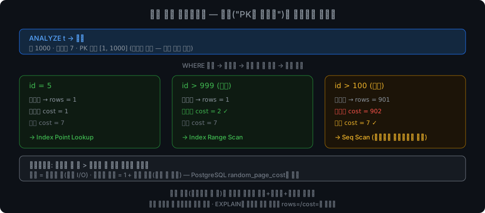
비용 기반 옵티마이저: ANALYZE 통계와 선택도로 매칭 행 수를 추정하고, 순차 vs 인덱스 비용을 비교해 싼 쪽을 고른다. 크로스오버는 페치 행 수가 페이지 수를 넘는 지점

세 번째 줄이 핵심입니다. 규칙 기반이라면 인덱스를 골랐을 자리에서, 비용 모델이 “901번 페치보다 7번 순차가 싸다”를 계산해 일부러 인덱스를 안 씁니다. 그리고 어느 경로든 결과 집합은 똑같습니다. 옵티마이저는 어떻게 가느냐만 바꾸지 무엇이 나오느냐는 안 바꿉니다(두 경로의 결과 동일성이 회귀 테스트). 단, 행이 나오는 순서는 다를 수 있습니다. ORDER BY 없이 “어쩌다 정렬돼 나오던” 순서에 기대던 코드가 플랜 변경 한 번에 깨지는 게 흔한 사고입니다.

흔한 오해 정정: “플랜은 인덱스 스캔이냐 풀스캔이냐 둘 중 하나다”. PostgreSQL엔 제3의 길이 있습니다. Bitmap Index Scan + Bitmap Heap Scan: 인덱스에서 매칭 RID를 전부 모아 페이지 순서로 정렬한 뒤, 힙을 순서대로 한 번씩만 방문합니다. 랜덤 페치의 저주를 정렬로 풀어서, 애매한 중간 선택도(인덱스는 아깝고 풀스캔은 과한 구간)의 기본 선택지가 됩니다. db-hobby에 이게 없는 건 RID를 모아 정렬하는 인프라가 없어서입니다. 그래서 db-hobby의 크로스오버는 실제 PostgreSQL보다 이분법적입니다.

실무/면접 포인트: “인덱스를 걸었는데 왜 안 타요?”의 절반이 이 이야기다. 옵티마이저가 통계를 보고 “이 쿼리는 대부분을 읽으니 순차가 싸다”고 판단한 것이다. 나머지 절반은 “통계가 오래돼(ANALYZE 안 됨) 플래너가 오판”이고. EXPLAIN의 rows= 추정치가 실제와 크게 다르면 그게 통계 문제의 신호다. 덧붙여 SSD 환경에선 random_page_cost를 기본 4.0에서 1.1 근처로 내리는 게 관례다. 4:1이라는 비율이 회전 디스크의 시크 시간에서 왔는데, SSD에선 랜덤과 순차의 차이가 거의 사라졌기 때문이다. 스캔 종류별 이론은 DB 인덱스 ②: 스캔의 종류와 옵티마이저의 선택.

이때 추정과 실측을 한 화면에서 대조하는 도구가 EXPLAIN ANALYZE입니다. 플랜만 출력하지 않고 실제로 실행해서 추정 rows=와 실측 actual rows를 나란히 보여줍니다(BUFFERS를 붙이면 페이지 접근 횟수까지). 둘이 크게 벌어진 노드가 바로 통계가 거짓말한 지점입니다.

흔한 오해 정정: “인덱스를 안 타면 힌트로 강제하면 된다”. 순서가 틀렸습니다. 먼저 ANALYZE로 통계를 갱신하고, EXPLAIN ANALYZE로 추정과 실측의 괴리를 확인하고, 조건이 sargable한지(컬럼에 함수·캐스트가 씌워져 인덱스를 못 쓰게 됐는지) 점검한 다음에야 비용 파라미터를 만질 차례입니다. 그리고 PostgreSQL엔 옵티마이저 힌트가 설계 철학상 없습니다(pg_hint_plan은 서드파티 확장). Oracle·MySQL·SQL Server가 힌트를 제공하는 것과 대비되는 지점입니다.

실무 안티패턴: 대량 적재 직후 ANALYZE 없이 서비스에 투입하는 것(통계가 빈 테이블 시절 그대로라 플래너가 전부 오판한다), 그리고 WHERE date_trunc('day', created_at) = ...처럼 컬럼을 함수로 감싸는 것(그 인덱스를 쓸 수 없게 된다. created_at >= ... AND created_at < ...로 풀어 쓰는 게 정석).

4. 조인 순서: 순서 하나가 2.8배를 가른다

단일 테이블은 “인덱스냐 순차냐”가 전부지만, 다중 테이블에선 옵티마이저의 진짜 고민이 나옵니다. 어느 순서로 조인하나. 세 테이블 체인으로 봅시다:

1
R0(1만 행) —[선택도 0.001]— R1(1천 행) —[선택도 0.01]— R2(10 행)

쿼리에 적힌 순서(R0부터)로 실행하면 큰 테이블끼리 먼저 만나 중간 결과가 커지고, 그걸 다음 단계가 또 처리합니다. 반대로 작은 R2부터 붙이면 중간 결과가 100으로 작게 유지됩니다. 같은 결과, 같은 세 테이블인데 순서만 바꿔 비용이 2.8배 줄어듭니다(db-hobby 비용 모델 기준).

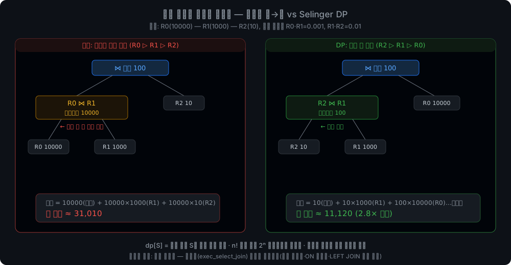
순진한 좌→우 순서 vs Selinger DP: 작은 테이블부터 붙여 중간 결과를 작게 유지

조인 순서의 본질: 최종 결과는 순서와 무관하지만, 중간 결과의 크기는 순서가 정한다. 옵티마이저의 일은 중간 결과를 작게 유지하는 순서를 찾는 것.

n!을 2ⁿ으로: Selinger의 부분집합 DP

테이블 n개의 순서는 n!가지입니다. 10개면 360만, 12개면 4억 8천만. 다 해볼 수 없습니다. 1979년 System R 논문에서 Patricia Selinger가 낸 답이 부분집합 동적 계획법입니다.

“관계 집합 S를 조인하는 최적 계획”은 S에서 하나 뺀 부분집합의 최적 계획에 그 하나를 붙인 것들 중 가장 싼 것이다. 이것이 최적 부분 구조다.

부분집합을 비트마스크로 표현하면({R0,R2} = 0b101), 채울 칸이 n!이 아니라 2ⁿ개입니다. 12개면 4억이 아니라 4096칸.

1
for (int mask = 1; mask <= full; mask++) {       /* 증가하는 정수 순서 = 작은 집합부터 */
2
    for (int r = 0; r < n; r++) {
3
        if (mask & (1 << r)) continue;
4
        double ncost = dp_cost[mask] + join_step_cost(g, mask, r, ...);
5
        int nmask = mask | (1 << r);
6
        if (ncost < dp_cost[nmask]) {
7
            dp_cost[nmask] = ncost;
8
            dp_prev[nmask] = mask;                /* 역추적용 */
9
        }
10
    }
11
}

mask를 증가하는 정수 순서로 훑는 게 트릭입니다. 어떤 부분집합(비트 하나 뺀 것)도 값이 더 작아 이미 확정돼 있으니, 위상 정렬이 필요 없습니다. 다 채운 뒤 dp_prev를 거꾸로 따라가면 최적 순서가 나옵니다. Selinger 논문의 유산이 하나 더 있습니다. interesting orders입니다. 정렬 순서를 만들어 두면 뒤의 ORDER BY나 머지 조인이 공짜가 되니, “지금은 조금 비싸도 유용한 순서를 가진 계획”을 부분해로 함께 보존한다는 아이디어입니다.

품질을 가르는 두 규칙

DP 뼈대만으론 부족합니다.

교차곱을 피하라(연결성): 조인 술어가 없는 두 관계를 붙이면 중간 결과가 |A|×|B|로 터집니다. 그래서 이미 조인된 집합에 조인 간선으로 연결된 관계만 다음 후보로 삼습니다(정말 분리된 그래프일 때만 교차곱을 허용하고 정직하게 표시).
방법까지 고른다: 각 확장 단계에서 인덱스 NLJ(안쪽에 인덱스가 있으면 프로브 ≈ 1)와 해시 조인(빌드+프로브)의 비용을 비교해 싼 방법을 그 단계에 기록합니다. 순서와 방법이 한 DP에서 같이 정해집니다.

검증은 성질로 합니다. “DP는 절대 순진한 좌→우 순서보다 나쁘지 않다”를 무작위 그래프 다수로 확인합니다(같은 비용 모델에서 DP 비용 ≤ 순진 비용이 불변식).

정직한 경계: 이 조인 순서 계획기는 독립 모듈이다. 실행기에 배선하려면 다중 테이블 통계·중간 결과 카디널리티 추정이 실행기 쪽에 있어야 한다. 단일 테이블 CBO(2~3절)는 실행기에 배선돼 있고, 조인 순서는 뼈대의 증명까지. PostgreSQL도 같은 계열의 부분집합 DP를 쓰는데(left-deep만이 아니라 bushy 트리까지 후보에 넣는 더 넓은 탐색), 표준 탐색은 FROM 항목 11개까지고, geqo_threshold(기본 12)개부터는 유전 알고리즘(GEQO)으로 넘어간다. 2ⁿ도 커지면 감당이 안 되기 때문이다.

조인 순서 탐색도 DB마다 전략이 갈립니다:

	조인 순서 탐색
PostgreSQL	부분집합 DP(bushy 포함). FROM 항목 12개(`geqo_threshold`)부터 GEQO(유전 알고리즘), `join_collapse_limit`(기본 8)로 탐색 단위 제한
MySQL	greedy 탐색. `optimizer_search_depth`로 깊이 조절(0이면 자동)
Oracle	비용 기반 순서 탐색 + 힌트(`LEADING` 등)와 adaptive plan으로 실행 중 보정

5. 정리

EXPLAIN의 원칙: 실행기와 같은 결정 함수를 공유한다. 플랜은 거짓말하지 않는다.
규칙이 틀리는 지점: db-hobby 모델에선 페치할 행 > 페이지 수면 순차가 이긴다. PostgreSQL은 random_page_cost(기본 4:1)·correlation·캐시가 크로스오버를 정하고, 중간 지대엔 Bitmap Scan이라는 제3의 길이 있다. “인덱스를 걸었는데 왜 안 타요?”의 정답.
CBO의 세 재료: ANALYZE(통계: db-hobby는 풀스캔, PG는 샘플링) → 선택도(균등분포 가정, 히스토그램·MCV·확장 통계는 그 다음) → 비용 비교. 통계 없으면 규칙으로 폴백.
조인 순서: 중간 결과 크기가 전부다. Selinger DP가 n!을 2ⁿ으로, 연결성 규칙이 교차곱을 막고, 방법(NLJ vs 해시)까지 한 DP에서. PostgreSQL은 FROM 항목 12개부터 GEQO로 넘어간다.

다음 편은 저장 엔진의 세 철학을 다룹니다. 힙(PostgreSQL) vs 클러스터드(InnoDB) vs LSM(RocksDB)을 한 코드베이스에서 실측으로 대조합니다.

참고 (1차 자료 우선)

P. G. Selinger et al., Access Path Selection in a Relational Database Management System (SIGMOD 1979): System R 옵티마이저 논문
Viktor Leis et al., How Good Are Query Optimizers, Really? (VLDB 2015): 카디널리티 추정 오차의 실측 벤치마크
PostgreSQL Documentation: Planner/Optimizer
PostgreSQL Documentation: Statistics Used by the Planner
PostgreSQL Documentation: Using EXPLAIN
PostgreSQL Documentation: Genetic Query Optimizer
본 블로그: DB 인덱스 ①: EXPLAIN 읽기 · ②: 스캔의 종류
db-hobby 코드 (GitHub): db.c(ANALYZE·비용 선택) · joinopt.c(Selinger DP)